9.14: Numerical Solutions for the Double Morse Potential

Last updated
Save as PDF

Page ID: 137732

\( \newcommand{\vecs}[1]{\overset { \scriptstyle \rightharpoonup} {\mathbf{#1}} } \) \( \newcommand{\vecd}[1]{\overset{-\!-\!\rightharpoonup}{\vphantom{a}\smash {#1}}} \)\(\newcommand{\id}{\mathrm{id}}\) \( \newcommand{\Span}{\mathrm{span}}\) \( \newcommand{\kernel}{\mathrm{null}\,}\) \( \newcommand{\range}{\mathrm{range}\,}\) \( \newcommand{\RealPart}{\mathrm{Re}}\) \( \newcommand{\ImaginaryPart}{\mathrm{Im}}\) \( \newcommand{\Argument}{\mathrm{Arg}}\) \( \newcommand{\norm}[1]{\| #1 \|}\) \( \newcommand{\inner}[2]{\langle #1, #2 \rangle}\) \( \newcommand{\Span}{\mathrm{span}}\) \(\newcommand{\id}{\mathrm{id}}\) \( \newcommand{\Span}{\mathrm{span}}\) \( \newcommand{\kernel}{\mathrm{null}\,}\) \( \newcommand{\range}{\mathrm{range}\,}\) \( \newcommand{\RealPart}{\mathrm{Re}}\) \( \newcommand{\ImaginaryPart}{\mathrm{Im}}\) \( \newcommand{\Argument}{\mathrm{Arg}}\) \( \newcommand{\norm}[1]{\| #1 \|}\) \( \newcommand{\inner}[2]{\langle #1, #2 \rangle}\) \( \newcommand{\Span}{\mathrm{span}}\)\(\newcommand{\AA}{\unicode[.8,0]{x212B}}\)

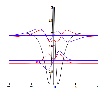
Schrödinger's equation is integrated numerically for the first four energy states for the double Morse oscillator. The integration algorithm is taken from J. C. Hansen, J. Chem. Educ. Software, 8C2, 1996.

Set parameters:

n = 200

xmin = -10

xmax = 10

\[ \Delta = \frac{xmax - xmin}{n-1} \nonumber \]

\( \mu\) = 1

D = 2

\( \beta\) = 1

x₀ = 1

Calculate position vector, the potential energy matrix, and the kinetic energy matrix. Then combine them into a total energy matrix.

i = 1 .. n j = 1 .. n x_i = xmin + (i - 1) \( \Delta\)

\[ V_{i,~j} = if \bigg[ i =j,~ D \big[ 1 - exp \big[ - \beta (|x_i| - x_0) \big] \big] ^2 ,~0 \bigg] \nonumber \]

\[ T_{i,~j} = if \bigg[ i=j, \frac{ \pi ^{2}}{6 \mu \Delta ^{2}}, \frac{ (-1)^{i-j}}{ (i-j)^{2} \mu \Delta^{2}} \bigg] \nonumber \]

Hamiltonian matrix: H = T + V

Find eigenvalues: E = sort(eigenvals(H))

Display four eigenvalues: m = 1 .. 4

E_m =

\( \begin{array}{|r|}
\hline \\
0.8092 \\
\hline \\
0.9127 \\
\hline \\
1.8284 \\
\hline \\
1.8975 \\
\hline
\end{array} \)

Calculate associated eigenfunctions:

k = 1 .. 4

\[ \psi (k) = eigenvec (H, E_k) \nonumber \]

Plot the potential energy and bound state eigenfunctions:

\[ Vpot_i = V_{i,~i} \nonumber \]

Screen Shot 2019-02-06 at 7.32.57 PM.png