9.8: Numerical Solutions for a Particle in a V-Shaped Potential Well

Last updated
Save as PDF

Page ID: 135870

\( \newcommand{\vecs}[1]{\overset { \scriptstyle \rightharpoonup} {\mathbf{#1}} } \) \( \newcommand{\vecd}[1]{\overset{-\!-\!\rightharpoonup}{\vphantom{a}\smash {#1}}} \)\(\newcommand{\id}{\mathrm{id}}\) \( \newcommand{\Span}{\mathrm{span}}\) \( \newcommand{\kernel}{\mathrm{null}\,}\) \( \newcommand{\range}{\mathrm{range}\,}\) \( \newcommand{\RealPart}{\mathrm{Re}}\) \( \newcommand{\ImaginaryPart}{\mathrm{Im}}\) \( \newcommand{\Argument}{\mathrm{Arg}}\) \( \newcommand{\norm}[1]{\| #1 \|}\) \( \newcommand{\inner}[2]{\langle #1, #2 \rangle}\) \( \newcommand{\Span}{\mathrm{span}}\) \(\newcommand{\id}{\mathrm{id}}\) \( \newcommand{\Span}{\mathrm{span}}\) \( \newcommand{\kernel}{\mathrm{null}\,}\) \( \newcommand{\range}{\mathrm{range}\,}\) \( \newcommand{\RealPart}{\mathrm{Re}}\) \( \newcommand{\ImaginaryPart}{\mathrm{Im}}\) \( \newcommand{\Argument}{\mathrm{Arg}}\) \( \newcommand{\norm}[1]{\| #1 \|}\) \( \newcommand{\inner}[2]{\langle #1, #2 \rangle}\) \( \newcommand{\Span}{\mathrm{span}}\)\(\newcommand{\AA}{\unicode[.8,0]{x212B}}\)

Schrödinger's equation is integrated numerically for a particle in a V-shaped potential well. The integration algorithm is taken from J. C. Hansen, J. Chem. Educ. Software, 8C2, 1996.

Set parameters:

n = 100 xmin = -4 xmax = 4 \( \Delta = \frac{xmax - xmin}{n-1}\) \( \mu\) = 1 Vo = 2

Calculate position vector, the potential energy matrix, and the kinetic energy matrix. Then combine them into a total energy matrix.

i = 1 .. n j = 1 .. n x_i = xmin + (i - 1) \( \Delta\)

V_{i, i} = V_o |x_i| T_i,j = if \( \bigg[ i=j, \frac{ \pi ^{2}}{6 \mu \Delta ^{2}}, \frac{ (-1)^{i-j}}{ (i-j)^{2} \mu \Delta^{2}} \bigg]\)

Hamiltonian matrix: H = T + V

Calculate eigenvalues: E = sort(eigenvals(H))

Selected eigenvalues: m = 1 .. 6

E_m =

\( \begin{array}{|r|}
\hline \\
1.284 \\
\hline \\
2.946 \\
\hline \\
4.093 \\
\hline \\
5.153 \\
\hline \\
6.089 \\
\hline\\
7.030 \\
\hline
\end{array} \)

Display solution:

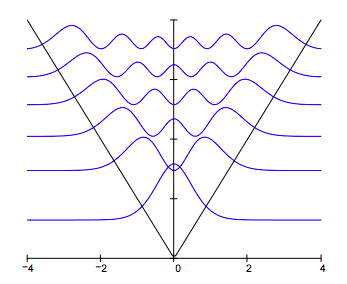
Screen Shot 2019-02-06 at 7.32.57 PM.png

For V = axⁿ the virial theorem requires the following relationship between the expectation values for kinetic and potential energy: <T> = 0.5n<V>. The calculations below show the virial theorem is satisfied for this potential for which n = 1.

\( \begin{pmatrix}
"Kinetic~Energy" & "Potential~Energy" & "Total~Energy" \\
\psi (1)^{T} T \psi(1) & \psi (1)^{T} V \psi(1) & E_{1} \\
\psi (2)^{T} T \psi(2) & \psi (2)^{T} V \psi(2) & E_{2} \\
\psi (3)^{T} T \psi(3) & \psi (3)^{T} V \psi(3) & E_{3}
\end{pmatrix} = \begin{pmatrix}
"Kinetic~Energy" & "Potential~Energy" & "Total~Energy" \\
0.428 & 0.857 & 1.284 \\
0.982 & 1.964 & 2.946 \\
1.365 & 2.728 & 4.093
\end{pmatrix} \)