9.5: Particle in a Finite Potential Well
- Page ID
- 135867

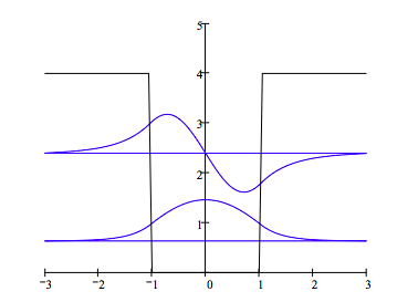
Numerical Solutions for the Finite Potential Well
Schrödinger's equation is integrated numerically for the first three energy states for a finite potential well. The integration algorithm is taken from J. C. Hansen, J. Chem. Educ. Software, 8C2, 1996.
Set parameters:
| n = 100 | xmin = -3 | xmax = 3 | \( \Delta = \frac{ xmax - xmin}{n-1}\) |
| \( \mu\) = 1 | lb = -1 | rb = 1 | V0 = 4 |
Calculate position vector, the potential energy matrix, and the kinetic energy matrix. Then combine them into a total energy matrix.
| i = 1 .. n | j = 1 .. n | xi = xmin + (i - 1) \( \Delta\) |
\( V_{i,i} = if[ (x_{i} \geq lb) (x_{i} \leq rb), 0, V_{0}]\) \( T_{i, j} = if [i=j, \frac{ \pi^{2}}{6 \mu \Delta^{2}}, \frac{(-1)^{i-j}}{(i-j)^{2} \mu \Delta^{2}} ]\)
Form Hamiltonian energy matrix: H = TV
Find eigenvalues: E = sort(eigenvals(H))
Display three eigenvalues: m = 1 .. 3
Em =
\( \begin{array}{|r|}
\hline \\
0.63423174 \\
\hline \\
2.39691438 \\
\hline \\
4.4105828 \\
\hline
\end{array} \)
Calculate associated eigenfunctions: k = 1 .. 2 \( \psi\)(k) = eigenvec(H, Ek)
Plot the potential energy and bound state eigenfunctions: \( V_{pot1} := V_{i,i}\)