Chemistry LibreTexts

9.1: Introduction to Numerical Solutions of Schödinger's Equation

  • Page ID
    135863
  • \( \newcommand{\vecs}[1]{\overset { \scriptstyle \rightharpoonup} {\mathbf{#1}} } \) \( \newcommand{\vecd}[1]{\overset{-\!-\!\rightharpoonup}{\vphantom{a}\smash {#1}}} \)\(\newcommand{\id}{\mathrm{id}}\) \( \newcommand{\Span}{\mathrm{span}}\) \( \newcommand{\kernel}{\mathrm{null}\,}\) \( \newcommand{\range}{\mathrm{range}\,}\) \( \newcommand{\RealPart}{\mathrm{Re}}\) \( \newcommand{\ImaginaryPart}{\mathrm{Im}}\) \( \newcommand{\Argument}{\mathrm{Arg}}\) \( \newcommand{\norm}[1]{\| #1 \|}\) \( \newcommand{\inner}[2]{\langle #1, #2 \rangle}\) \( \newcommand{\Span}{\mathrm{span}}\) \(\newcommand{\id}{\mathrm{id}}\) \( \newcommand{\Span}{\mathrm{span}}\) \( \newcommand{\kernel}{\mathrm{null}\,}\) \( \newcommand{\range}{\mathrm{range}\,}\) \( \newcommand{\RealPart}{\mathrm{Re}}\) \( \newcommand{\ImaginaryPart}{\mathrm{Im}}\) \( \newcommand{\Argument}{\mathrm{Arg}}\) \( \newcommand{\norm}[1]{\| #1 \|}\) \( \newcommand{\inner}[2]{\langle #1, #2 \rangle}\) \( \newcommand{\Span}{\mathrm{span}}\)\(\newcommand{\AA}{\unicode[.8,0]{x212B}}\)

    Solving Schrödinger's equation is the primary task of chemists in the field of quantum chemistry. However, exact solutions for Schrödinger's equation are available only for a small number of simple systems. Therefore the purpose of this tutorial is to illustrate one of the computational methods used to obtain approximate solutions.

    Mathcad offers the user a variety of numerical differential equation solvers. We will use Mathcad's ordinary differential equation solver, Odesolve, because it allows one to type Schrödinger's equation just as it appears on paper or on the blackboard; in other words it is pedagogically friendly. In what follows the use of Odesolve will be demonstrated for the one-dimensional harmonic oscillator. All applications of Odesolve naturally require the input of certain parameters: integration limits, mass, force constant, etc. Therefore the first part of the Mathcad worksheet will be reserved for this purpose.

    • Integration limit: xmax := 5
    • Effective mass: µ := 1
    • Force constant: k := 1

    The most important thing distinguishing one quantum mechanical problem from another is the potential energy term, \(V(x)\). It is entered below.

    Potential energy:

    \[ V(x) = \dfrac{1}{2} kx^{2} \nonumber \]

    Entering the potential energy separately, as done above, allows one to write a generic form for the Schrödinger equation applicable to any one-dimensional problem. This creates a template that is easily edited when moving from one quantum mechanical problem to another. All that is necessary is to type in the appropriate potential energy expression and edit the input parameters. This is the most valuable feature of the numerical approach - you don't need a new mathematical tool or trick for each new problem, a single template works for all one-dimensional problems after minor editing.

    Mathcad's syntax for solving the Schrödinger equation is given below. As it may be necessary to do subsequent calculations, the wavefunction is normalized. Note that seed values for an initial value for the wavefunction and its first derivative are required. It is also important to note that the numerical integration is carried out in atomic units:

    \[h/2π = me = e = 1. \nonumber \]

    Given

    \[ \frac{-1}{2 \mu} \frac{d^{2}}{dx^{2}} \psi (x) + V(x) \psi (x) = E \psi (x) \nonumber \]

    with \( \psi (-x_{max}) = 0\) and \( \psi '(-x_{max}) = 0.1\).

    \[ \psi = Odesolve (x, x_{max}) \nonumber \]

    Normalize wavefunction:

    \[ \psi (x) = \frac{ \psi (x)}{\displaystyle \sqrt{ \int_{-x_{max}}^{x_{max}} \psi (x)^{2} dx}} \nonumber \]

    Numerical solutions also require an energy guess. If the correct energy is entered the integration algorithm will generate a wavefunction that satisfies the right-hand boundary condition. If the right boundary condition is not satisfied another energy guess is made. In other words it is advisable to sit on the energy input place holder, type a value and press F9 to recalculate.

    Energy guesses that are too small yield wavefunctions that miss the right boundary condition on the high side, while high energy guesses miss the right boundary condition on the low side. Therefore it is generally quite easy to bracket the correct energy after a few guesses.

    Enter energy guess: E ≡ .5

    Of course the solution has to be displayed graphically to determine whether a solution (an eigenstate) has been found. The graphical display is shown below. It is frequently instructive to also display the potential energy function.
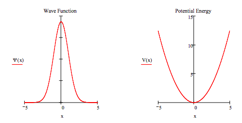
    Screen Shot 2019-02-06 at 12.19.38 PM.png

    wavefunction:

    %matplotlib inline
    
    from scipy.integrate import odeint
    import matplotlib.pyplot as plt  
    import numpy as np
    
    
    mu=1
    k=1
    E=.5
    xmax=-5
    
    def psi(y,x):
        psi1, psi2_dx2 = y 
        return [psi2_dx2, ((2*mu)/(-1))*(E*psi1 - (1/2)*x**2*psi1)]
    
    x0 = [0.0, 0.1]
    val = np.linspace(-5,5,101)
    sol = odeint(psi, x0, val)
    #plot, legends, and titles 
    plt.plot(val,sol[:,0],color = "red",label = " ")
    plt.title("Wave Function")
    leg = plt.legend(title = "(x)  ", loc = "center", bbox_to_anchor=[-.11,.5],frameon=False)
    
    plt.show()
    

    Potential energy:

    %matplotlib inline  
    
    import matplotlib.pyplot as plt
    import numpy as np
    import math
    
    # initialize constants k and create x array
    k = 1 
    x = np.linspace(-5,5,100)
    
    # set boundaries
    plt.xticks([-5,5])
    plt.yticks([0,5,10,15])
    
    # plot
    plt.plot(x,(.5)*k*(x**2), color = "red",label = " ")
    
    # add titles and legend
    plt.title("Potential Energy")
    leg = plt.legend(title = "\u03A8  ", loc = "center", bbox_to_anchor=[-.11,.5],frameon=False)
    
    plt.show()
    

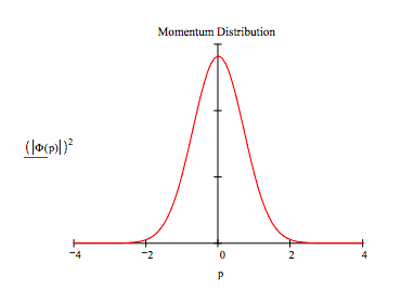
    It is quite easy, as shown below, to generate the momentum-space wavefunction by a Fourier transform of its coordinate-space counterpart.

    \( p := -4, -3.9..5\)

    \[ \Phi (p) = \frac{1}{ \sqrt{ 2 \pi}} \int_{-x_{max}}^{x_{max}} e^{-i p x} \psi(x)dx \nonumber \]

    Screen Shot 2019-02-06 at 12.19.46 PM.png

    %matplotlib inline  
    
    import numpy as np
    import matplotlib.pyplot as plt 
    from scipy.integrate import odeint
    import scipy.integrate as integrate
    import math
    
    #set constants
    mu=1
    k=1
    E=.5
    xmax=5
    
    #create ode 
    def psi(y,x):
        psi1, psi2_dx2 = y 
        return [psi2_dx2, ((2*mu)/(-1))*(E*psi1 - (1/2)*x**2*psi1)]
    
    #create space 
    x0 = [0.0, 0.001]
    val = np.linspace(-xmax,xmax,101)
    
    #solve ode using odeint
    sol = odeint(psi, x0, val)
    
    #format plot
    fig = plt.figure()
    ax = fig.add_subplot(1, 1, 1)
    
    #show tick marks to the left and lower axes only
    plt.yticks([])
    plt.axis(xmin = -4,xmax = 4,ymin = 0,ymax = 30)
    
    #move left yaxis passing through origin
    ax.spines["left"].set_position("center")
    
    #eliminate upper and right axes
    ax.spines["right"].set_color("none")
    ax.spines["top"].set_color("none")
    
    #plot graph
    plt.plot(val,sol[:,0],color = "red",label = " ")
    
    
    #add titles and legend
    plt.title("Momentum Distribution")
    leg = plt.legend(title = "(|\u03A6(p)|\u00b2)", loc = "center", bbox_to_anchor=[-.10,.5],frameon=False)
    
    plt.show()


    This page titled 9.1: Introduction to Numerical Solutions of Schödinger's Equation is shared under a CC BY 4.0 license and was authored, remixed, and/or curated by Frank Rioux via source content that was edited to the style and standards of the LibreTexts platform; a detailed edit history is available upon request.