9.13: Numerical Solutions for the Lennard-Jones Potential

Last updated
Save as PDF

Page ID: 137731

\( \newcommand{\vecs}[1]{\overset { \scriptstyle \rightharpoonup} {\mathbf{#1}} } \) \( \newcommand{\vecd}[1]{\overset{-\!-\!\rightharpoonup}{\vphantom{a}\smash {#1}}} \)\(\newcommand{\id}{\mathrm{id}}\) \( \newcommand{\Span}{\mathrm{span}}\) \( \newcommand{\kernel}{\mathrm{null}\,}\) \( \newcommand{\range}{\mathrm{range}\,}\) \( \newcommand{\RealPart}{\mathrm{Re}}\) \( \newcommand{\ImaginaryPart}{\mathrm{Im}}\) \( \newcommand{\Argument}{\mathrm{Arg}}\) \( \newcommand{\norm}[1]{\| #1 \|}\) \( \newcommand{\inner}[2]{\langle #1, #2 \rangle}\) \( \newcommand{\Span}{\mathrm{span}}\) \(\newcommand{\id}{\mathrm{id}}\) \( \newcommand{\Span}{\mathrm{span}}\) \( \newcommand{\kernel}{\mathrm{null}\,}\) \( \newcommand{\range}{\mathrm{range}\,}\) \( \newcommand{\RealPart}{\mathrm{Re}}\) \( \newcommand{\ImaginaryPart}{\mathrm{Im}}\) \( \newcommand{\Argument}{\mathrm{Arg}}\) \( \newcommand{\norm}[1]{\| #1 \|}\) \( \newcommand{\inner}[2]{\langle #1, #2 \rangle}\) \( \newcommand{\Span}{\mathrm{span}}\)\(\newcommand{\AA}{\unicode[.8,0]{x212B}}\)

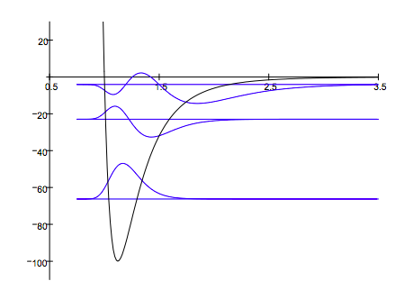
Merrill (Am. J. Phys. 1972, 40, 138) showed that a Lennard-Jones 6-12 potential with these parameters had three bound states. This is verified by numerical integration of Schrödinger's equation. The integration algorithm is taken from J. C. Hansen, J. Chem. Educ. Software, 8C2, 1996.

Set parameters:

n = 200
\(x_{min} = 0.75\)
\(x_{max} = 3.5\)
\(\Delta = \frac{xmax - xmin}{n-1}\)
\( \mu\) = 1
\( \sigma\) = 1
\( \varepsilon\) = 100

Numerical integration algorithm:

i = 1 .. n j = 1 .. n x_i = xmin + (i - 1) \( \Delta\)

\[ V_{i,~j} = if \bigg[ i =j,~4 \varepsilon \bigg[ \left( \frac{ \sigma}{x_i} \right)^12 - \left( \frac{ \sigma}{x_i} \right) ^6 \bigg] ,0~ \bigg] \nonumber \]

\[ T_{i,~j} = if \bigg[ i=j, \frac{ \pi ^{2}}{6 \mu \Delta ^{2}}, \frac{ (-1)^{i-j}}{ (i-j)^{2} \mu \Delta^{2}} \bigg] \nonumber \]

Hamiltonian matrix: H = T + V

Find eigenvalues: E = sort(eigenvals(H))

Display three eigenvalues: m = 1 .. 4

E_m =

\( \begin{array}{|r|}
\hline \\
-66.269 \\
\hline \\
-22.981 \\
\hline \\
-4.132 \\
\hline \\
1.096 \\
\hline
\end{array} \)

Calculate eigenvectors:

k = 1 .. 3

\[ \psi (k) = eigenvec (H, E_k) \nonumber \]

Display results:

Screen Shot 2019-02-06 at 7.32.57 PM.png