9.9: Numerical Solutions for the Harmonic Oscillator

Last updated
Save as PDF

Page ID: 137727

\( \newcommand{\vecs}[1]{\overset { \scriptstyle \rightharpoonup} {\mathbf{#1}} } \) \( \newcommand{\vecd}[1]{\overset{-\!-\!\rightharpoonup}{\vphantom{a}\smash {#1}}} \)\(\newcommand{\id}{\mathrm{id}}\) \( \newcommand{\Span}{\mathrm{span}}\) \( \newcommand{\kernel}{\mathrm{null}\,}\) \( \newcommand{\range}{\mathrm{range}\,}\) \( \newcommand{\RealPart}{\mathrm{Re}}\) \( \newcommand{\ImaginaryPart}{\mathrm{Im}}\) \( \newcommand{\Argument}{\mathrm{Arg}}\) \( \newcommand{\norm}[1]{\| #1 \|}\) \( \newcommand{\inner}[2]{\langle #1, #2 \rangle}\) \( \newcommand{\Span}{\mathrm{span}}\) \(\newcommand{\id}{\mathrm{id}}\) \( \newcommand{\Span}{\mathrm{span}}\) \( \newcommand{\kernel}{\mathrm{null}\,}\) \( \newcommand{\range}{\mathrm{range}\,}\) \( \newcommand{\RealPart}{\mathrm{Re}}\) \( \newcommand{\ImaginaryPart}{\mathrm{Im}}\) \( \newcommand{\Argument}{\mathrm{Arg}}\) \( \newcommand{\norm}[1]{\| #1 \|}\) \( \newcommand{\inner}[2]{\langle #1, #2 \rangle}\) \( \newcommand{\Span}{\mathrm{span}}\)\(\newcommand{\AA}{\unicode[.8,0]{x212B}}\)

Schrödinger's equation is integrated numerically for the first three energy states for the harmonic oscillator. The integration algorithm is taken from J. C. Hansen, J. Chem. Educ. Software, 8C2, 1996.

Set parameters:

Increments: n = 100

Integration limits: xmin = -5

xmax = 5

\[ \Delta = \frac{xmax - xmin}{n-1} \nonumber \]

Effective mass: \( \mu\) = 1

Force constant: k = 1

Calculate position vector, the potential energy matrix, and the kinetic energy matrix. Then combine them into a total energy matrix.

i = 1 .. n j = 1 .. n x_i = xmin + (i - 1) \( \Delta\)

\[ V_{i,~j} = if \bigg[ i =j,~ \frac{1}{2} k (x)^2 ,~0 \bigg] \nonumber \]

\[ T_{i,~j} = if \bigg[ i=j, \frac{ \pi ^{2}}{6 \mu \Delta ^{2}}, \frac{ (-1)^{i-j}}{ (i-j)^{2} \mu \Delta^{2}} \bigg] \nonumber \]

Hamiltonian matrix: H = T + V

Find eigenvalues: E = sort(eigenvals(H))

Display three eigenvalues: m = 1 .. 3

E_m =

\( \begin{array}{|r|}
\hline \\
0.5000 \\
\hline \\
1.5000 \\
\hline \\
2.5000 \\
\hline
\end{array} \)

Calculate associated eigenfunctions:

k = 1 .. 3

\[ \psi (k) = eigenvec (H, E_k) \nonumber \]

Plot the potential energy and selected eigenfunctions:

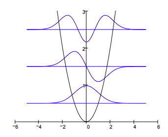
Screen Shot 2019-02-06 at 7.32.57 PM.png

For V = axⁿ the virial theorem requires the following relationship between the expectation values for kinetic and potential energy: <T> = 0.5n<V>. The calculations below show the virial theorem is satisfied for the harmonic oscillator for which n = 2.

\( \begin{pmatrix}
"Kinetic~Energy" & "Potential~Energy" & "Total~Energy" \\
\psi (1)^{T} T \Psi(1) & \psi (1)^{T} V \psi(1) & E_{1} \\
\psi (2)^{T} T \Psi(2) & \psi (2)^{T} V \psi(2) & E_{2} \\
\psi (3)^{T} T \Psi(3) & \psi (3)^{T} V \psi(3) & E_{3}
\end{pmatrix} = \begin{pmatrix}
"Kinetic~Energy" & "Potential~Energy" & "Total~Energy" \\
0.2500 & 0.2500 & 0.5000 \\
0.7500 & 0.7500 & 1.5000 \\
1.2500 & 1.2500 & 2.5000
\end{pmatrix} \)