11.13: Simple Kinetic Derivations of Thermodynamic Relations

Introduction

Kinetics and thermodynamics seem like very different disciplines. They emphasize different phenomena (change; equilibrium) and introduce different concepts (rate constants; energy/entropy). It is not widely known that a useful connection between those disparate fields was suggested late in the 19^th century by Svante Arrhenius when he introduced the concept of the activated molecule to account for the exponential dependence on temperature of kinetic rate constants (1,2). Textbook accounts of Arrhenius's rate-constant law fail to reveal the creative use Arrhenius made of thermodynamic principles in his analysis of the temperature dependence of chemical reaction rates, and, thus, fail to exploit Arrhenius's insights into the teaching of thermodynamics.

After a brief review of Arrhenius's work, we will show that the relations of classical thermodynamics of chief interest to chemists can be obtained by simple algebra from elementary rate laws and Arrhenius's rate constant expression

\[ k = Ae^{ \frac{ \Delta H^{*}}{RT}} \nonumber \]

The Origin of Arrhenius's Rate Constant Expression (1)

Facts: Reaction rate have significant temperature dependencies (typically on the order of +8 percent per degree), which cannot be accounted for by increase gas-phase collision frequencies or decreased liquid-phase viscocities.

For all practical purposes, the concentration of reactant molecules are not temperature dependent.

Hypothesis: Since the concentration of a reactant (M) does not vary with temperature, the actual reactant species (in a unimolecular reaction) might be an activated form of the molecule M^*, with

\[ Rate = \mathcal{K} (M^{*}) \nonumber \]

where the constant \( \mathcal{K}\) is independent of temperature and (M^*) is directly proportional to (M) and is sharply dependent on temperature.

\[ (M^{*}) = k(T)~(M) \nonumber \]

Implications: Relationship 471.3 can be substituted into 471.2

\[ Rate = \mathcal{K} k(T)~(M) \nonumber \]

which emphasizes that k(T) is a kinetic rate parameter. Relationship 471.3 can be rewritten as

\[ k(T) = \frac{(M^{*})}{(M)} \nonumber \]

which emphasizes that k(T) is, also, a thermodynamic parameter: an equilibrium constant. As such it satisfies van 't Hoff's expression¹

\[ \frac{d \ln( k(T))}{dT} = \frac{ \Delta H^{*}}{RT^{2}} \nonumber \]

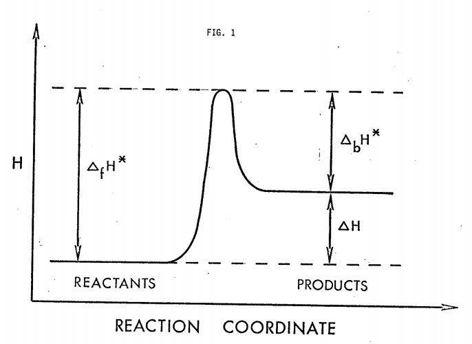
where \( \Delta H^{*}\) is the enthalpy change accompanying the formation of M^* from M - the enthalpy of activation. If over small intervals \( \Delta H^{*}\) may be treated as a constant, the integrated form of Equation 471.6 is essentially expression 471.1: \( k(T) = Ae^{ - \Delta H^{*} \ RT}\), where A is a constant independent of T. As indicated in Figure 1 (f = forward, b = backward),

\[ \Delta_{f} H^{*} = \Delta_{b} H^{*} = \Delta H \Delta E + \Delta (PV) \nonumber \]

Discussion: Thermodynamics played a large role in Arrhenius's elucidation of the temperature dependence of rate constants. It is not surprising, then, that the relations of classical thermodynamics can be obtained from elementary rate laws and Arrhenius's rate-constant expression. Below are eight illustrative examples of simple kinetic derivations of thermodynamic relations.

¹Arrhenius employed van 't Hoff's equation in the form \( \frac{ d( \ln(k)}{dT} = \frac{q}{RT^{2}}\). Under the usual conditions of constant pressure \( q = \Delta H\). This accounts for our use of \( \Delta H^{*}\) rather than E_a in equation 471.1.

Clapeyron's Equation for Condensed Phases

In this analysis and those that follow, the simplest mechanism consistent with overall stoichiometry is employed. It is not difficult to show that more complicated mechanisms would yield the same result (see paper cited by Frost in footnote 2).

For equilibrium with respect to the change:

\( x_{(solution)} \underset{k_b}{\stackrel{k_f}{\rightleftharpoons}} x_{(pure~liquid)}\)

R_f (melting rate) = k_f = R_b (freezing rate) = k_b. The concentrations of pure substances are constant and therefore absorbed in the rate constants. Thus, by equation 471.1, at equilibrium

\( A_{f} e^{ \frac{- \Delta_{f} H^{*}}{RT}} = A_{b} e^{ \frac{- \Delta_{b} H^{*}}{RT}}\)

Hence, by equation 471.7, on taking logarithms,

\( \frac{ \Delta E + P \Delta V}{RT} = \ln( \frac{A_{f}}{A_{b}}) = constant\)

For equilibrium to be maintained when T and P change from values satisfying the above expression to new values T + dT and P + dP, dT and dP must be such that

\( \frac{ \Delta E~+~(P + dP)~ \Delta V}{R (T + dT)} = \frac{ \Delta E~+~P \Delta V}{RT}\)

Simplification yields Clapeyron's equation

\[ \frac{dP}{dT} = \frac{ \Delta H}{T \Delta V} \nonumber \]

Ideal Solubility and Freezing Point Depression

For equilibrium with respect to the change

\( x_{(solid)} \underset{k_b}{\stackrel{k_f}{\rightleftharpoons}} x_{(ideal~solution)}\)

R_f (melting or solution rate) = k_f = R_b (freezing or precipitation rate) = k_bN_x. Thus, by equations 471.1 and 471.7, for all mole fractions N_x,

\( \ln( \frac{A_{f}}{A_{b}} = \frac{ \Delta H}{RT} + \ln(N_{x}) = \frac{ \Delta H}{RT} |_{N_{x} = 1} = \frac{\Delta H}{RT_{nfp}}\).

Hence,

\[ \ln(N_{x}) = \frac{ \Delta H}{R} ( \frac{1}{T_{nfp} - \frac{1}{T}}) = \frac{ \Delta H (T - T_{nfp})}{RTT_{nfp}} \nonumber \]

For \( N_{x} \cong 1\), \(T \cong T_{nfp}\) (of x), \( \ln(N_{x} \cong N_{x} - 1 \cong N_{2}\) and

\[ -(T-T_{nfp}) \cong \frac{RT^{2}_{nfp}}{ \Delta H} N_{2} \nonumber \]

Osmotic Equilibrium

For equilibrium with respect to the change

\( x_{(pure~liquid)} \underset{k_b}{\stackrel{k_f}{\rightleftharpoons}} x_{(ideal~solution)}\)

	Pure Liquid	Ideal Solution
Pressure	P	P + \( \pi \)
Mole Fraction	Nx = 1	Nx < 1

R_f = k_f = R_b = k_bN_x. Thus, by equations 471.1 and 471.7,

\( ln \frac{A_{f}}{A_{b}} = \frac{ \Delta E~+~ \Delta (PV)}{RT} + \ln(N_{x})\)

In this instance:

\( \Delta E = \Delta V = 0\)

\( \Delta (PV) = (P + \pi) \overline{V}_{x} - P \overline{V}_{x} = \pi \overline{V}_{x}\).

Hence,

\( \frac{A_{f}}{A_{b}} = \frac{ \pi \overline{V}_{x}}{RT} + \ln(N_{x})\).

For N_x = 1, \( \pi\) = 0. Thus \( \ln( \frac{A_{f}}{A_{b}}) = 0\).

Hence,

\[ \pi = - \frac{RT}{ \overline{V}_{x}} \ln(N_{x}) \cong \frac{RTN_{2}}{ \overline{V}_{x}} \cong RTC_{2} \nonumber \]

where N₂ << 1.

Chemical Equilibrium

For equilibrium with respect to the change

aA + bB = cC + dD

the Principle of Microscopic Reversibility states that the rate at which A and B disappear by the (perhaps unlikely) mechanism aA + bB, rate law R_f = k_fc_A^ac_B^b, is equal to the rate at which A and B appear by the mechanism cC + dD, rate law R_b = k_bc_C^cc_D^d.² Thus, with equations 471.1 and 471.7, one obtains

\[ K \equiv \frac{c_{C}^{c}}{C_{D}^{d}} |_{equilibrium} = \frac{k_{f}}{k_{b}} = \frac{A_{f}}{A_{b}} e^{ \frac{- \Delta H}{RT}} \nonumber \]

or,

\[ \ln(K) + \frac{ \Delta H}{RT} = \ln( \frac{A_{f}}{A_{b}}) = constant \nonumber \]

If T changes from T₁ to T₂, the change in K, from K₁ to K₂, must be such that, by equation 471.12,

\[ \ln( \frac{K_{2}}{K_{1}}) = \frac{ \Delta H}{R} (\frac{1}{T_{1}} - \frac{1}{T_{2}}) \nonumber \]

²For a further discussion of this point, see Frost, A. A. and Pearson, R. G., "Kinetics and Mechanism," John Wiley and Sons, Inc., 1953, Ch. 8; or Frost, A. A., J. Chem. Educ., 18, 272 (1941).

Boltzmann's Factor

For equilibrium with respect to the simple "chemical" change

\( x~(quantum~state~i) \underset{b}{\stackrel{f}{\rightleftharpoons}} x~(quantum~state~j)\)

one has by 471.11,

\( K = \frac{C_{j}}{C_{i}} = \frac{A_{f}}{A_{b}} e^{ \frac{- \Delta H}{RT}}\)

In this instance:

\( A_{f} = A_{b}\)

\( \Delta H = \Delta E~+~P \Delta V = \Delta E \equiv N_{A}( \varepsilon_{j} - \varepsilon_{i})\).

\( \frac{C_{j}}{C_{i}} = \frac{N_{j}}{N_{i}}\)

Hence,

\[ \frac{N_{j}}{N_{i}} = e^{ \frac{- ( \varepsilon_{j} - \varepsilon_{i})}{kT}} \nonumber \]

Electrochemical Equilibrium

For equilibrium with respect to the flow of electrons in an electrochemical circuit

\( e~(potential~V_{1}) \underset{k_b}{\stackrel{k_f}{\rightleftharpoons}} e~(potential~V_{2})\)

R_f = k_f = R_b = k_b. Thus, by equation 471.1,

\( \ln \frac{A_{f}}{A_{b}} = \frac{ \Delta_{f} H^{*} - \Delta_{b} H^{*}}{RT}\)

The activation enthalpies contain in this instance two contributions: one from the enthalpy of activation of the chemical change to which the electron flow is coupled in an electrochemical cell; the other from the enthalpy of activation for the physical transfer of electrons across a potential difference E = V₁ - V₂. In this instance, \( \Delta_{f} H^{*} - \Delta_{b} H^{*} = \Delta H + nFE \).

Hence,

\( \ln \frac{A_{f}}{A_{b}} = \frac{ \Delta H + nFE}{RT}\).

For equilibrium to be maintained when T and E change from values satisfying the above expression to new values T + dT and E + dE, dT and dE must be such that

\( \frac{ \Delta H + nF(E~+~dE)}{R(T~+~dT)} = \frac{ \Delta H + nFE}{RT}\)

Simplification yields

\( nF \frac{dE}{dT} = \frac{ \Delta H + nFE}{T}\)

By the First Law, \( \Delta H + nFE = Q_{rev}\).

Hence,

\[ nF \frac{dE}{dT} = \frac{Q_{rev}}{T} \nonumber \]

Equation 471.16 is a special instance of the general thermodynamic relation

\[ \frac{dW_{rev}}{dT} = \frac{Q_{rev}}{T} \nonumber \]

Alternatively: \[ \frac{dW_{rev}}{Q_{rev}} = \frac{dT}{T} \nonumber \]

[In Gibbs-Clausius notation: \( \frac{ \delta ( \Delta G)}{ \delta T} = - \Delta S\)]

Equation 471.18 is, in turn, a special instance of the Kelvin-formula for the efficiency of a reversible heat engine.

\[ \varepsilon_{rev} = \frac{T_{2} - T_{1}}{T_{2}} \nonumber \]

Mechanical Equilibrium

For equilibrium with respect to a change, in the energy E of a purely mechanical system say a change in altitude, h, of a weight, wt,

\[ wt(E_{i} = Mgh_{i}) \underset{b}{\stackrel{f}{\rightleftharpoons}} wt(E_{j} = Mgh_{j}), \nonumber \]

R_f = k_f = R_b = k_b. Hence, by equations 471.1, 471.7 with, again, A_f = A_b,

\[ \frac{R_{f}}{R_{b}} = \frac{k_{f}}{k_{b}} = e^{ \frac{- (E_{j} - E_{i})}{kT}} = e^{- \Delta E_{wt}}{kT} \nonumber \]

For, for example, \( \Delta h\) = +0.1m, M = 0.05 kg, and g = 9.8 \( \frac{m}{s^{2}}\), \( \Delta E_{wt}\) = +0.0049 J. Thus, at T = 300K (k = 1.38 x 10^-23 J),

\( \frac{R_{f}}{R_{b}} = 10^{-(10^{18.7})}\)

Boltzmann's Relation

For change 471.20 let the number of macroscopically indistinguishable, microscopically distinct quantum states accessible jointly to the mechanical system wt and its thermal surroundings \( \theta\) in (wt + \( \theta\))'s initial state i, its transition state *, and its final state j be denoted, respectively, \( ( \Omega_{total})_{i}\), \( ( \Omega_{total}^{*})\), and \( ( \Omega_{total})_{j} \). If all quantum states are, a priori, equally probably, \( R_{f} = k \frac{ ( \Omega_{total})^{*}}{( \Omega_{total})_{i}}\) and \( R_{b} = k \frac{ ( \Omega_{total})^{*}}{( \Omega_{total})_{j}}\). Thus, for equilibrium with respect to change 471.20, by 471.21,

\[ \frac{ ( \Omega_{total})_{j}}{( \Omega_{total})_{i}} = e^{ \frac{ \Delta E_{wt}}{kT}} \nonumber \]

By the First Law, for a universe wt + \( \theta\), \( - \Delta_{wt} = \Delta E_{ \theta}\). By the Second Law, \( \frac{ \Delta E_{ \theta}}{T} = \Delta S_{ \theta}\). By the law of statistical independence, \( \Omega_{total} = \Omega_{ \theta} \Omega_{wt}\). And by the law of the reversibility of purely mechanical changes, \( \Omega_{wt}\) = constant. Thus, by equation 471.22,

\[ \frac{ ( \Omega_{ \theta} )_{final}}{( \Omega_{ \theta} )_{initial}} = e^{ \frac{ \Delta S_{ \theta}}{k}} \nonumber \]

By the Third Law, S = 0 when \( \Omega = 1\) (for example, a perfect crystal at T = 0K). Thus, by equation 471.23, for systems in internal equilibrium,

\[ S = k \ln \Omega \nonumber \]

Summary and Concluding Comments

Arrhenius's expression (equation 471.1) embodies in a form immediately applicable to chemical problems those implications of the Second-Law-like behavior of Nature of particular interest to chemists. It is, from a chemical point of view, a more quickly and easily used expression of the Second Law than is the more widely applicable but, though mathematically simpler, chemically more remote expression 471.19.

Expression 1 is in a certain sense, said Arrhenius, "a paraphrase of the observed facts" (1). It is an axiomatization of a nearly universal feature of chemical reactions. If chemical (and physical) changes had no enthalpies of activation, it would be impossible to store energy - as, for example, fat or fuel plus oxygen. Everything would slide quickly to equilibrium, including the sun. Without energy barriers there would be no life - and energy crises.

Arrhenius's expression 1 is based on van 't Hoff's thermodynamic expression \( K = Ce^{ \frac{- \Delta H}{RT}}\) (1, 2). Thus, the kinetic derivations above are not, in a logical sense, substitutes for thermodynamic arguments. It is often instructive, however, to see abstract expressions emerge unexpectedly from concrete, special instances.

The present mathematical procedures can be used without change in purely thermodynamic arguments. From the expression \( K = Ce^{ \frac{- \Delta H}{RT}}\) one can obtain quickly, as above, expressions 471.8-471.16 without using calculus, the entropy function, the chemical potential, or Carnot's cycle.

Conventional expressions that involve the entropy function can be obtained from the present discussion by introducing the abbreviation \( \Delta S \equiv R \ln \frac{A_{f}}{A_{b}}\).

Literature Cited

1. Arrhenius, S., Z. Physik Chem., 4, 226 (1889); excerpted and translated by Back, M. H. and Laidler, K. J., "Selected Readings in Chemical Kinetics," Pergamon Press, New York, 1967, pp. 31-35.

2. van 't Hoff, J. H., "Studies in Chemical Dynamics," translated by Thomas Ewan, Chemical Publishing Co., Easton, Pennsylvania, 1896, pp. 122-123.