5.26: X-ray Diffraction

This tutorial on X‐ray diffraction was stimulated by an appendix in the first edition of Peter Atkinsʹ celebrated physical chemistry text (pp. 734‐739) titled ʺDiffraction as a particle property.ʺ In exploring this approach we will work in one dimension in the interests of mathematical and conceptual simplicity.

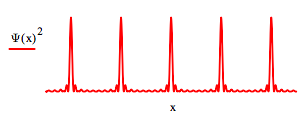
Modeling the periodicity of the electron density in a one‐dimensional atomic lattic requires the superposition of many electron wavelengths and, therefore, by the de Broglie relation (λ = h/p) many electron momentum states. For example, a superposition of eight cosine functions yields the sharply defined electron density distribution with lattice spacing d shown below.

\[ \begin{matrix} d=1 & \Psi (x) = \sum_{n=1}^8 \cos \left( n 2 \pi \frac{x}{d} \right) \end{matrix} \nonumber \]

where d is the lattice spacing and λ = d/n with n = 1, 2, 3...

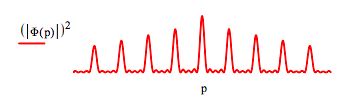
According to the quantum mechanical interpretation of diffraction, when this one‐dimensional electron density distribution interacts with an X‐ray source the individual photons are temporarily localized simultaneously at all lattice sites. The uncertainty principle requires that spatial localization leads to a delocalization (scattering) of the momentum distribution and the appearance of interference fringes because the spatial localization occurs at multiple sites. The resulting momentum distribution is the diffraction pattern and is calculated by a Fourier transform of the electron density distribution, Ψ(x)², into momentum space as is shown below (in atomic units: h = 2π).

\[ \Phi (p) = \frac{1}{ \sqrt{2 \pi}} \int_{-.5}^{4.5} \Psi (x)^2 exp(ipx)dx \nonumber \]

The approach adopted by Atkins is to model diffraction as an elastic particle‐like collision between the X‐ray photon and the electron distribution of the lattice. In this view one asks what momenta the lattice can transfer to the incident particle (photon). The quantum mechanical answer to this question is provided by the scattering amplitude or structure factor shown in the following equation.

\[ F(p') = \int \langle p-p' | \Psi \rangle \langle \Psi | p \rangle dp \nonumber \]

Reading the Dirac brackets above from right to left, this expression is the scattering amplitude or the ʺpossibilityʺ that an electronic state Ψ with momentum p can transfer momentum pʹ to the scattered particle. Integrating the brackets over p yields all the ways that the electron distribution represented by Ψ can transfer momentum pʹ to the incident photon.

The structure factor can be cast into the coordinate representation by applying the completeness relation

\[ \int | x \rangle \langle x | dx = 1 \nonumber \]

to the left bracket in the integral followed by rearrangement.

\[ F(p') = \int \int \langle p-p' |x \rangle \langle x | \Psi \rangle \langle \Psi | p \rangle dxdp \nonumber \]

Using the momentum eigenfunction in the coordinate representation and the position eigenfunction in the momentum representation (normalization constants are ignored throughout this treatment),

\[ \langle x|p \rangle = \langle p|x \rangle* = \text{exp} \left( \frac{ipx}{ \hbar} \right) \nonumber \]

we see that the middle bracket on the right can be transformed as follows,

\[ \langle p - p" | x \rangle = \text{exp} \left( \frac{-i (p-p')x}{ \hbar} \right) = \text{exp} \left( - \frac{ipx}{ \hbar} \right) \text{exp} \left( \frac{ip'x}{ \hbar} \right) = \langle p | x \rangle \langle x | p' \rangle \nonumber \]

F(p') can now be written as

\[ F(p') = \int \int \langle \Psi | p \rangle \langle p|x \rangle \langle x | p' \rangle \langle x| \Psi \rangle dxdp \nonumber \]

Using the momentum-space completeness relation,

\[ \int |p \rangle \langle p | dp = 1 \nonumber \]

we find,

\[ F(p') = \int \langle \Psi | x \rangle \langle x | p' \rangle \langle x | \Psi \rangle dx \nonumber \]

Expressing F(p') in traditional notation yields,

\[ F(p') = \int \Psi* (x) \text{exp} \left( \frac{ip'x}{ \hbar} \right) \Psi (x) dx = \int \rho (x) \text{exp} \left( \frac{ip'x}{ \hbar} \right) dx \nonumber \]

Note that we have reached the same point as in our initial approach: Fourier transform the electron density into the momentum representation to calculate the diffraction pattern.

We conclude by recovering the traditional form of the structure factor found in all physical chemistry texts and books dealing with X‐ray crystallography. The momenta, pʹ, that the electron distribution can transfer to the incident photon are the momenta that it has.

Earlier it was noted that to build a one‐dimensional electron density distribution with lattice spacing d requires the superposition of wavelengths restricted by the relation λ = d/n, where n = 1,2,3, ... This requires, by de Broglieʹs wave equation, a superposition of quantized momentum states given by pʹ = nh/d. Substitution of this equation into F(pʹ) yields

\[ F(n) = \int \rho \text{exp} \left( 2 \pi i \frac{nx}{d} \right) dx \nonumber \]

where n is the Miller index that normally goes by the designation h. The extension to three dimensions using the traditional (h, k, l) designation for the Miller indices, and a, b and c for the lattice constants is straightforward.