5.9: Calculating Diffraction Patterns

I wish to describe a simple extension of Marcella’s [1] recent analysis of the double-slit experiment to two dimensions.

The essential point Marcella makes in his unique treatment of this well-known experiment is that the diffraction pattern at the detection screen is actually a measurement of the momentum distribution of the diffracted particles. Therefore the calculated diffraction pattern is simply obtained from the Fourier transform of the coordinate space wave function (the double-slit geometry) into momentum space. Marcella considered two spatial models: (1) infinitesimally thin slits represented by Dirac delta functions, and (2) slits of finite width.

About sixty years ago Sir Lawerence Bragg [2] proposed the optical transform as an aid in the interpretation of the x-ray diffraction patterns of crystals. This required the fabrication of two-dimensional masks of various crystal or molecular geometries and the generation of the diffraction pattern using visible electromagnetic radiation. Present day laser technology has made the generation of such diffraction patterns routine, even in the classroom.

In addition, Marcella’s computational approach makes calculating the diffraction patterns conceptually and mathematically straightforward. If one considers the mask as consisting of point scatterers (model 1), the coordinate space wave function is a linear superposition of the scattering positions,

\[ | \Psi \rangle = \frac{1}{ \sqrt{N}} \sum_{i = 1}^N |x_i,~y_1 \rangle \nonumber \]

where N is the number of point scatterers.

The Fourier transform into the momentum representation yields,

\[ \langle p | \Psi \rangle = \frac{1}{ \sqrt{N}}_{i=1}^N \langle p_x | x_i \rangle \langle p_y | y_i \rangle = \frac{1}{2 \pi h \sqrt{N}} \sum_{i = 1}^N exp \left[ - \frac{i}{h} (p_xx_i + p_yy_i) \right] \nonumber \]

For model 2, which assumes finite-sized scatterers, equation (2) becomes,

\[ \langle p | \Psi \rangle = \frac{1}{2 \pi h r \sqrt{N}} \sum_{i = 1}^N \int_{x_i - \frac{r}{2}}^{x_i + \frac{r}{2}} exp \left[ - \frac{ip_xx}{h} \right] dx \int_{y_i - \frac{r}{2}}^{y_i + \frac{r}{2}} exp \left[ - \frac{ip_y y}{h} \right] dy \nonumber \]

where r is the spatial dimension of the scatterers. In the interest of mathematical simplicity, the scatterers are assumed to be small squares rather than circles.

Figure 1 shows the diffraction pattern, \(| \langle p | \Psi \rangle |^2\), for a hexagonal arrangement of six point scatterers calculated using equation (2), while figure 2 shows the pattern obtained with equation (3) for six finite hexagonal scatterers. The calculated diffraction pattern shown in figure 2 is in excellent agreement with the experimental diffraction pattern available in the literature [3]. The calculations [4] of the diffraction patterns were carried out in atomic units (h = 2π) so that positions are given in a0 and momenta in a0 -1. The distance between adjacent scatters is 1.4 a0 and their spatial dimension is 0.3 a0 on a side.

Figure 1. Diffraction pattern for a hexagonal arrangement of six point scatterers.

Figure 2. Diffraction pattern for a hexagonal arrangement of six finite scatterers.

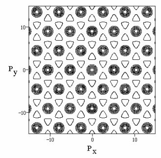
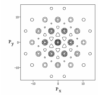
In addition to showing the interference effects accompanying scattering from multiple positions, the figures also illustrate the uncertainty principle. Figure 1 shows no attenuation of the diffraction pattern at extreme values of momentum because the point scatterers sharply localize the particle being scattered in coordinate space, leading to a delocalized momentum distribution as required by the position-momentum uncertainty relation. By comparison the finite scatterers of figure (2) lead to some uncertainty in position and, therefore, less uncertainty in momentum. Therefore the diffraction pattern is attenuated at large values for both the x- and y-momentum components.

References

1. Marcella T V 2002 Eur. J. Phys. 23 615-621
2. Bragg L 1944 Nature 154 69-72
3. Harburn G, Taylor C A and Welberry T R 1975 Atlas of Optical Transforms (Ithaca, NY: Cornell University Press) Plates 4 and 5.
4. The Mathcad 5.0 files used to generate Figures 1 and 2 are available for download at ww.users.csbsju.edu/frioux/di.../hex-point.mcd and ~/hex-finite.mcd.