
3.36: Posch-Teller Potential Model for Metals
- Page ID
- 154843

The purpose of this tutorial is to use a one‐dimensional Posch‐Teller potential to model the electronic behavior of metals. Schrödingerʹs equation is integrated numerically for the first six energy states, producing two bands of bound states separated by a significant band gap. The integration algorithm is taken from J. C. Hansen, J. Chem. Educ. Software, 8C2, 1996.)
\[ \begin{matrix} \text{Set parameters:} & n = 200 & xmin = -6 & xmax = 6 & \Delta = \frac{xmax - xmin}{n-1} \\ \mu = 1 & Vo = -10 & \alpha = 2 & d = 2 & a = 1 \end{matrix} \nonumber \]
Calculate the position vector, the potential energy matrix, and the kinetic energy matrix. Then combine them into a total energy matrix.
\[ \begin{matrix} i = 1 .. n & j = 1 .. n & x_i = xmin + (i-1) \Delta \end{matrix} \nonumber \]
\[ \begin{matrix} V_{i,~j} = \text{if} \left[ \right] & T_{i,~j} = \text{if} \left[ i = j,~ \frac{ \pi^2}{6 \mu \Delta^2},~ \frac{(-1)^{i-j}}{(i-j)^2 \mu \Delta^2} \right] \end{matrix} \nonumber \]
Total energy matrix: H = T + V
Calculate eigenvalues: \( \text{E = sort(eigenvals(H))}\)
Display selected eigenvalues: m = 1 .. 6
\[ E_m = \begin{array}{|c|} \hline -6.5283 \\ \hline -6.4484 \\ \hline -6.3942 \\ \hline -1.8562 \\ \hline -1.3274 \\ \hline -0.6173 \\ \hline \end{array} \nonumber \]
Calculate eigenvectors: \( \begin{matrix} k = 1 .. 6 & \Psi (k) = \text{eigenvec} \left( H,~E_k \right) \end{matrix}\)
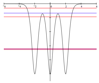
Display the potential energy and energy eigenvalues to show band formation:
Display the potential energy and electron density distributions offset by an arbitrary amount for purposes of clarity:
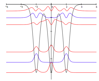
Discussion of the model: The metal cations occupy the potential energy minima. The electron density distributions show that the allowed valence electron states are delocalized over the metal structure. Delocalization is achived (especially for the lower energy band) by quantum tunneling through the internal energy barriers representing the inter‐nuclear regions.
Bunching of the allowed energy states into two ʺbandsʺ separated by a significant band gap occurs because the states have different electron densities at the locations of the potential energy minima and maxima, in addition to the fact that kinetic energy increases with increasing quantum number. This is illustrated by the following table in which the expectation values for kinetic and potential energy are calculated. Note that the kinetic energy always increases with increasing quantum number, but within a band the potential energy actually decreases slightly.
\[ \begin{pmatrix} \text{"Kinetic Energy"} & \text{"Potential Energy"} & \text{"Total Energy"} \\ \Psi (1)^T T \Psi (1) & \Psi (1)^T V \Psi (1) & E_1 \\ \Psi (2)^T T \Psi (2) & \Psi (2)^T V \Psi (2) & E_2 \\ \Psi (3)^T T \Psi (3) & \Psi (3)^T V \Psi (3) & E_3 \\ \Psi (4)^T T \Psi (4) & \Psi (4)^T V \Psi (4) & E_4 \\ \Psi (5)^T T \Psi (5) & \Psi (5)^T V \Psi (5) & E_5 \\ \Psi (6)^T T \Psi (6) & \Psi (6)^T V \Psi (6) & E_6 \\ \end{pmatrix} = \begin{pmatrix} \text{"Kinetic Energy"} & \text{"Potential Energy"} & \text{"Total Energy"} \\ 1.1917 & -7.7201 & -6.5283 \\ 1.3766 & -7.8251 & -6.4484 \\ 1.5634 & -7.9576 & -6.3942 \\ 1.924 & -3.7855 & -1.8562 \\ 2.4726 & -3.8000 & -1.3274 \\ 3.2362 & -3.8535 & -0.6173 \end{pmatrix} \nonumber \]