3.34: Semi-empirical Molecular Orbital Calculation on HF

Calculate the wavefunctions and energies of the σ orbitals in the HF molecule, taking β = -1.0 eV. The values of the Coulomb integrals αH and αF are taken as the negatives of the orbital ionization energies of the atoms.

The molecular orbital is formed as a linear combination of the valence orbitals of H and F.

\[ \Psi = C_h \Psi_h + C_f \Psi_f \nonumber \]

where

\[ \Psi_h = 1s(h) and \Psi_f = 2p_z (f) \nonumber \]

The variational integral for this calculation is,

\[ E = \frac{ \int_0^{ \infty} \left( C_h \Psi_h + C_f \Psi_f \right) H \left( C_h \Psi_h + C_h \Psi_f \right) d \tau}{ \int_0^{ \infty} \left( C_h \Psi_h + C_f \Psi_f \right)^2 d \tau} \nonumber \]

Minimization of the variational energy integral simultaneously with respect to Ch and Cf yields two linear homogeneous equations (see McQuarrie and Simon, section 7-2, for details).

\[ \begin{matrix} C_h \left[ H_{hh} - ES_{hh} \right] + C_f \left[ H_{hf} - ES_{hf} \right] = 0 \\ C_h \left[ H_{hf} - ES_{hf} \right] + C_f \left[ H_{ff} - ES_{ff} \right] = 0 \end{matrix} \nonumber \]

where the integral and their parameterizations are presented below.

\[ \begin{matrix} H_{hh} = \int_0^{ \infty} \Psi_h H \Psi_h d \tau = -13.6 & S_{hh} = \int_0^{ \infty} \Psi_h^2 d \tau = 1 \\ H_{ff} = \int_0^{ \infty} \Psi_f H \Psi_f d \tau = \alpha_f = -18.6 & S_{ff} = \int_0 ^{ \infty} \Psi_f^2 d \tau = 1 \\ H_{hf} = \int_0^{ \infty} \Psi_h H \Psi_f d \tau = \beta = -1 & Shf = \int_0^{ \infty} \Psi_h \Psi_f d \tau = 0 \end{matrix} \nonumber \]

In matrix form equations (4) can be written as,

\[ \begin{pmatrix} \alpha_h - E & \beta \\ \beta & \alpha_f - E \end{pmatrix} \begin{pmatrix} C_h \\ C_f \end{pmatrix} = \begin{pmatrix} 0 \\ 0 \end{pmatrix} \nonumber \]

or, as an eigenvalue equation,

\[ \begin{pmatrix} \alpha_h & \beta \\ \beta & \alpha_f \end{pmatrix} \begin{pmatrix} C_h \\ C_f \end{pmatrix} = \begin{pmatrix} E & 0 \\ 0 & E \end{pmatrix} \begin{pmatrix} C_h \\ C_f \end{pmatrix} \nonumber \]

Mathcad can now be used to find the eigenvalues and eigenvectors of (6). First we must give it the values for all the parameters.

\[ \begin{matrix} \alpha_f = -18.6 & \alpha_h = -13.6 & \beta = -1 \end{matrix} \nonumber \]

Define the variational matrix shown on the left side of equation (6):

\[ H = \begin{pmatrix} \alpha_h & \beta \\ \beta & \alpha_f \end{pmatrix} \nonumber \]

Find the eigenvalues:

\[ \begin{matrix} \text{E = sort(eigenvals(H))} & \text{E}_0 = -18.79 & E_1 = -13.41 \end{matrix} \nonumber \]

Now find the eigenvectors:

\[ \begin{matrix} \text{The bonding MO is:} & \Psi_h = \text{eigenvec} \left( H,~E_0 \right) & \Psi_b = \begin{pmatrix} 0.19 \\ 0.98 \end{pmatrix} & \overrightarrow{ \left( \Psi_b^2 \right)} = \begin{pmatrix} 0.04 \\ 0.96 \end{pmatrix} \\ \text{The anti-bonding MO is:} & \Psi_h = \text{eigenvec} \left( H,~E_1 \right) & \Psi_b = \begin{pmatrix} -0.98 \\ 0.19 \end{pmatrix} & \overrightarrow{ \left( \Psi_a^2 \right)} = \begin{pmatrix} 0.96 \\ 0.04 \end{pmatrix} \end{matrix} \nonumber \]

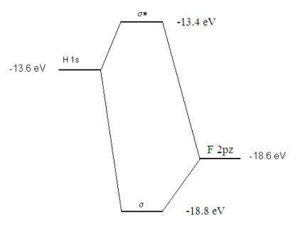
Squaring the coefficients of the wavefunction we find that an electron in the bonding molecular orbital spends 96% of its time on the fluorine atom and 4% of its time on the hydrogen atom. Because fluorine has a kernel charge (nuclear charge minus two non-valence electrons) of +7 and gets credit, according to the appended MO diagram for six non-bonding electrons, plus 96% of the two bonding electrons, the net charge on flourine can be shown to be -.92. This value indicates that the H-F bond is quite polar, which is consistent with the high electronegativity of the flourine atom.

On the Pauling scale the electronegativities of H and F are 2.1 and 4.0, respectively. The partial charge on H is calculated as: nuclear charge - non-valence electrons - unshared valence electrons - bonding electrons times χ_H/(χ_H + χ_F). As shown below these formal charge calculations do not give fluorine such a high negative charge.

\[ \begin{matrix} Z_H = 1 & _F = 9 & \chi_H = 2.1 & \chi_F = 4.0 \\ \delta_H = 1-0-0-2 \frac{ \chi_H}{ \chi_H + \chi_F} & \delta_H = 0.31 & \delta_F = 9 - 2 - 6 - 2 \frac{ \chi_F}{ \chi_H + \chi_F} & \delta_F = -0.31 \end{matrix} \nonumber \]

Mathcad offers another way of performing the variational calculation. The variational integral given in equation (3) can also be written in the following form in which the integrals have been replaced by the experimental parameters used to replace them.

\[ E = \frac{C_h^2 \alpha_h + C_f^2 \alpha_f + 2 C_h C_f \beta}{C_h^2 + C_f^2 + 2C_h C_f S_{hf}} \nonumber \]

This expression can be minimized simultaneously with respect to C_h and C_f in a Given/Find solve block. As is usually the case, Mathcad requires seed values or actual values for all the variables that appear in the solve block. There are two solutions, the ground state and the excited state. That is, the bonding molecular orbital and the anti-bonding molecular orbital. Within the solve block we have the equation for the energy, its first derivative with respect to C_h and C_f each set equal to zero, and the normalization requirement. To find the ground state we chose initial values of the coefficients that favor the fluorine 2p_z orbital.

\[ \begin{matrix} C_h = 0.1 & C_f = .9 & \alpha_h = -13.6 & \alpha_f = -18.6 & \beta = - 7 S_{hf} = 0 & E = -10 \end{matrix} \nonumber \]

Given

\[ \begin{matrix} E = \frac{C_h^2 \alpha_h + C_f^2 \alpha_f + 2C_h C_f \beta}{C_h^2 + C_f^2 2C_h S_{hf}} & \frac{d}{dC_h} \frac{C_h^2 \alpha_h + C_f^2 \alpha_f + 2C_h C_f \beta}{C_h^2 + C_f^2 2C_h S_{hf}} = 0 \\ \frac{d}{dC_f} \frac{C_h^2 \alpha_h + C_f^2 \alpha_f + 2C_h C_f \beta}{C_h^2 + C_f^2 2C_h S_{hf}} = 0 & C_h^2 + C_f^2 + 2C_h C_f S_{hf} = 1 \end{matrix} \nonumber \]

Given these constraints, we ask Mathcad to find a solution. The solution yields wavefunction coefficients and the ground-state energy.

\[ \text{Find} \left( C_h,~C_f,~E \right) = \begin{pmatrix} 0.19 \\ 0.98 \\ -18.79 \end{pmatrix} \nonumber \]

To find the anti-bonding state, we choose initial coefficients that favor the hydrogen 1s orbital.

\[ \begin{matrix} C_h = .9 & C_f = 0.1 & \alpha = -13.6 & \alpha_f = -18.6 & \beta = -1 & S_{hf} = 0 & E = -10 \end{matrix} \nonumber \]

Given

\[ \begin{matrix} E = \frac{C_h^2 \alpha_h + C_f^2 \alpha_f + 2C_h C_f \beta}{C_h^2 + C_f^2 2C_h S_{hf}} & \frac{d}{dC_h} \frac{C_h^2 \alpha_h + C_f^2 \alpha_f + 2C_h C_f \beta}{C_h^2 + C_f^2 2C_h S_{hf}} = 0 \\ \frac{d}{dC_f} \frac{C_h^2 \alpha_h + C_f^2 \alpha_f + 2C_h C_f \beta}{C_h^2 + C_f^2 2C_h S_{hf}} = 0 & C_h^2 + C_f^2 + 2C_h C_f S_{hf} = 1 \end{matrix} \nonumber \]

Given these constraints, we ask Mathcad to find a solution.

\[ \text{Find} \left( C_h,~F_f,~E \right) = \begin{pmatrix} 0.98 \\ -0.19 \\ -13.41 \end{pmatrix} \nonumber \]

There is yet another way that Mathcad can do this calculation that requires that the symbolic processor be loaded. Equation (5) in matrix form has a non-trivial solution only if the determinant of the coefficient matrix is equal to zero.

\( \begin{pmatrix} \alpha_h - E & \beta \\ \beta & \alpha_f - E \end{pmatrix}\) has determinant \( \alpha_h - \alpha_f - \alpha_h E - E \alpha_f + E^2 - \beta^2\) which has solution(s)

\[ \begin{pmatrix} \frac{1}{2} \alpha_h + \frac{1}{2} \alpha_f + \frac{1}{2} \sqrt{ \alpha_h^2 - 2 \alpha_h \alpha_f + \alpha_f^2 + 4 \beta^2} \\ \frac{1}{2} \alpha_h + \frac{1}{2} \alpha_f + \frac{1}{2} \sqrt{ \alpha_h^2 - 2 \alpha_h \alpha_f + \alpha_f^2 + 4 \beta^2} \end{pmatrix} = \begin{pmatrix} -13.41 \\ -18.79 \end{pmatrix} \nonumber \]

Find the bonding molecular orbital:

E = -18.793

Given \( \left( \alpha_h - E \right) C_h + \beta C_f = 0\) and \( \begin{matrix} C_h^2 + C_f^2 + 2C_h C_f S_{hf} =1 & \text{Find} \left( C_h,~C_f \right) = \begin{pmatrix} 0.19 \\ 0.98 \end{pmatrix} \end{matrix}\)

Find the anti-bonding molecular orbital:

E = -13.407

Given \( \left( \alpha_h - E \right) C_h + \beta C_f = 0\) and \( \begin{matrix} C_h^2 + C_f^2 + 2C_h C_f S_{hf} =1 & \text{Find} \left( C_h,~C_f \right) = \begin{pmatrix} 0.98 \\ -0.19 \end{pmatrix} \end{matrix}\)

The molecular orbital calculation can be summarized graphically as shown below.

Reference: See page 428 of Atkins and de Paula, Physical Chemistry, 7th edition.