3.29: A Numerical Huckel MO Calculation on C60

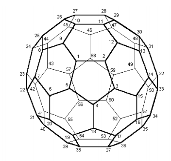
1. Number the carbons after inspection of the molecular structure and fill in data needed below.

\[ \begin{matrix} \text{Natoms = 60} & \text{the number of carbon atoms and } π- \text{electrons} \\ \text{Nocc = 30} & \text{the number of occupied molecular occupied} \end{matrix} \nonumber \]

2. Create a 60 x 60 null matrix.

\[ \begin{matrix} \text{i = 1 .. Natoms} & \text{j = 1 .. Natoms} & \text{H}_{i,~j} = 0 \end{matrix} \nonumber \]

3. Form the Huckel matrix from the null matrix using the results of part 1.

\[ \begin{matrix} \text{k = 1 .. Natoms - 1} & \text{H}_{k,~k+1} = 1 \end{matrix} \nonumber \]

\[ \begin{matrix} H_{1,~5} = 1 & H_{1,~9} = 1 & H_{2,~12} = 1 & H_{3,~15} = 1 & H_{4,~18} = 1 & H_{6,~20} = 1 & H_{7,~22} = 1 \\ H_{8,~25} = 1 & H_{10,~26} = 1 & H_{11,~29} = 1 & H_{13,~30} = 1 & H_{14,~33} = 1 & H_{16,~34} = 1 & H_{17,~37} = 1 \\ H_{19,~38} = 1 & H_{21,~40} = 1 & H_{23,~42} = 1 & H_{24,~44} = 1 & H_{27,~45} = 1 & H_{28,~47} = 1 & H_{31,~48} = 1 \\ H_{32,~50} = 1 & H_{35,~51} = 1 & H_{36,~53} = 1 & H_{39,~54} = 1 & H_{41,~55} = 1 & H_{43,~57} = 1 & H_{46,~58} = 1 \\ H_{49,~59} = 1 & H_{52,~60} = 1 & H_{56,~60} = 1 & H_{j,~i} = H_{i,~j} & H = -H\end{matrix} \nonumber \]

4. Calculate the eigenvalues and eigenvectors. It is not feasible to look at the eigenvectors as a group because that would require displaying a 60 x 60 matrix. The eigenvalues will be displayed later.

\[ \begin{matrix} \text{E = eigenvals(H)} & \text{C = submatrix} \left( \text{rsort} \left( \text{stack} \left( \text{E}^T,~ \text{eigenvecs(H)} \right), ~ 1 \right),~2 \text{Natoms +1, 1, Natoms} \right) \end{matrix} \nonumber \]

5. Use the eigenvectors to calculate selected π-electron densities and π-bond orders. If r = s you are calculating the π-electron density on carbon r. If r is not equal to s you are calculating the r-s π-bond order. Several examples are given below. These calculations can be used to show that all the carbons have the same π-electron density and that there are only two physically meaningful π-bond orders.

\[ \begin{matrix} r = 1 & s = 1 & 2 \sum_{i = 1}^{ \text{Nocc}} \left( C^{<i>} \right)_r,~ \left( C^{<i>} \right)_s = 1 & \pi- \text{electron density on carbon 1} \\ r = 1 & s = 2 & 2 \sum_{i = 1}^{ \text{Nocc}} \left( C^{<i>} \right)_r,~ \left( C^{<i>} \right)_s = 0.476 & \pi- \text{bond order between carbons 1 and 2} \\ r = 1 & s = 5 & 2 \sum_{i = 1}^{ \text{Nocc}} \left( C^{<i>} \right)_r,~ \left( C^{<i>} \right)_s = 0.476 & \pi- \text{bond order between carbons 1 and 5} \\ r = 1 & s = 9 & 2 \sum_{i = 1}^{ \text{Nocc}} \left( C^{<i>} \right)_r,~ \left( C^{<i>} \right)_s = 0.601 & \pi- \text{bond order between carbons 1 and 9} \end{matrix} \nonumber \]

Note that the π-bond order is higher for bonds that fuse two hexagons compared to bonds that fuse a hexagon and a pentagon.

6. Display the energy eigenvalues: \( \text{E = sort(E)}\)

\[ \begin{matrix} i = 1 .. 15 & E_i & i = 16 .. 30 & E_i & i = 31 .. 45 & E_i & i = 46 .. 60 & E_i \\ ~ & \begin{array}{|c|} \hline -3 \\ \hline -2.757 \\ \hline -2.757 \\ \hline -2.757 \\ \hline -2.303 \\ \hline -2.303 \\ \hline -2.303 \\ \hline -2.303 \\ \hline -2.303 \\ \hline -1.82 \\ \hline -1.82 \\ \hline -1.82 \\ \hline -1.562 \\ \hline -1.562 \\ \hline -1.562 \\ \hline \end{array} & ~ & \begin{array}{|c|} \hline -1.562 \\ \hline -1 \\ \hline -1 \\ \hline -1 \\ \hline -1 \\ \hline -1 \\ \hline -1 \\ \hline -1 \\ \hline -1 \\ \hline -1 \\ \hline -0.618 \\ \hline -0.618 \\ \hline -0.618 \\ \hline -0.618 \\ \hline -0.618 \\ \hline \end{array} & ~ & \begin{array}{|c|} \hline 0.139 \\ \hline 0.139 \\ \hline 0.139 \\ \hline 0.382 \\ \hline 0.382 \\ \hline 0.382 \\ \hline 1.303 \\ \hline 1.303 \\ \hline 1.303 \\ \hline 1.303 \\ \hline 1.303 \\ \hline 1.438 \\ \hline 1.438 \\ \hline 1.438 \\ \hline 1.618 \\ \hline \end{array} & ~ & \begin{array}{|c|} \hline 1.618 \\ \hline 1.618 \\ \hline 1.618 \\ \hline 1.618 \\ \hline 2 \\ \hline 2 \\ \hline 2 \\ \hline 2 \\ \hline 2.562 \\ \hline 2.562 \\ \hline 2.562 \\ \hline 2.562 \\ \hline 2.618 \\ \hline 2.618 \\ \hline 2.618 \\ \hline \end{array} \end{matrix} \nonumber \]

The energy eigenvalues can also be displayed graphically as follows: \(i = 1 .. 60\)

Attention should be drawn to the nine-fold degenerate state at E = -1. C₆₀ belongs to the icosahedral point group and the largest degeneracy permitted is 5-fold. Thus, this state is an example of the accidental degeneracy of a 5-fold degenerate state and a 4-fold degenerate state.

7. It is easy to show that this manifold of energy states is in agreement with the basic facts about C₆₀. For example, it is diamagnetic and a non-conductor. Placing the 60 π-electrons is the lowest available energy states completely fills all the bonding molecular orbitals. The HOMO has an energy of -.618 |β| and contains ten paired electrons giving a diamagnetic and non-conducting electronic structure. The LUMO is three-fold degenerate and not far away in energy. This is consistent with the fact that C₆₀ has a high electron affinity and forms ionic compounds with alkali metals such as potassium. For example, K₃C₆₀ (three unpaired electrons in the LUMO) is a conductor and becomes a superconductor at low temperatures, while K₆C₆₀ (six paired electrons in the LUMO) is a non-conductor.

The Huckel calculation can be extended with a simple example of modeling. Since the results of the following calculation require the assignment of a value for β, the results should not be taken too seriously. The HOMO-LUMO gap is .757 |β|. Giving |β| a typical value 2.5 eV enables one to calculate the wavelength of light required to promote an electron from the HOMO to the LUMO.

\[ \begin{matrix} eV = 1.6021777 (10)^{-19} \text{joule} & h = 6.62608 (10)^{-34} \text{joule sec} & c = 2.99792458 (10)^8 \frac{m}{sec} \\ \beta = 2.5 eV & nm = 10^{-9} m & \lambda = 1 nm \\ \text{Given} & \frac{hc}{ \lambda} = .757 | \beta | & \text{Find}( \lambda ) = 655 nm \end{matrix} \nonumber \]

This result is just barely within the visible region and not in particularly good agreement with a known visible transition around 400 nm. However, it should be noted that the HOMO-LUMO transition is formally forbidden. The HOMO-LUMO+1 is allowed and the energy gap is |β| which would give an optical transition at 496 nm, in better agreement with the experimental value.

There are a number of very weak features in the visible spectrum between 440 and 670 nm any of which may be attributable to the forbidden HOMO-LUMO transtion. However, it is also true that small amounts of other fullerenes may be contributing to this part of the visible spectrum.

8. Calculate the π-electron stabilization energy per carbon atom. This is calculated by summing the energies of the occupied orbitals and multiplying by two. Subtract from this the π-electron binding energy of the equivalent number of ethylene molecules and divide by the number of carbon atoms, which is the same as the number of π-electrons.

\[ \begin{matrix} \Delta E_{ \pi} = \frac{2 \sum_{i - 1}^{ \text{Nocc}} \left| E_i \right| - \text{Natoms}}{ \text{Natoms}} & \Delta E_{ \pi} = 0.553 \end{matrix} \nonumber \]

Recall that the π-electron stabilization energy per carbon atom for benzene is 0.333.