3.26: A Modified Tangent Spheres Model Analysis of Trigonal Bipyramidal Geometry

Why do non‐bonding electron pairs occupy the equatorial rather than the axial positions in trigonal bipyramidal geometry? VSEPR teaches that it is because they have more room in the equatorial positions and this leads to lower electron‐electron repulsion. The modified Tangent Spheres Model (TSM) [see Bent, H. A. J. Chem. Educ. 40, 446‐452 (1963) for an introduction] calculation below shows that equatorial electrons indeed have a lower energy than the axial electrons, but not for the reason VSEPR postulates.

In this modified TSM approach an electron is represented as a particle in a sphere of radius R. The wave function for such an electron is the eigenfunction of the kinetic energy operator in spherical coordinates, with energy π²/(2R²) in atomic units, as is shown below.

\[ \begin{matrix} \Phi (r,~R) = \frac{1}{ \sqrt{2 \pi R}} \frac{ \sin \left( \frac{ \pi r}{R} \right)}{r} & \frac{ - \frac{1}{2r} \frac{d^2}{dr^2} \left( r \Phi (r,~R) \right)}{\Phi (r,~R)} \rightarrow \frac{1}{2} \frac{ \pi^2}{R^2} \end{matrix} \nonumber \]

According to the Pauli Exclusion Principle each spherical wave function (orbital) can accomodate two electrons. These non‐interpenetrating Pauli spheres are surogates for the hybridized atomic orbitals that are frequently invoked in VSEPR explanations.

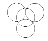
There are five such pairs (three equatorial and two axial) in trigonal bipyramidal geometry. The trigonal planar hole created by the equatorial electron pairs is occupied by the nuclear kernel (nucleus plus non‐valence electrons). The pockets created by the trigonal planar spheres are occupied by the two axial pairs of electrons. The equatorial electrons and one of the axial pairs is shown in the figure below.

In the calculations carried out here, the equatorial and axial electron spheres are allowed to have different radii. This means there are two variational parameters in the energy calculation, the radii of the axial and equatorial spherical electron clouds. The nuclear kernel is treated as +10 point charge centered in the trigonal planar hole, and its electrostatic interaction with the valence electrons is its only contribution to the total energy. The contributions to the energy are identified in the table below. These Mathcad calculations are carried out using atomic units.

\[ \begin{bmatrix} \text{Energy Contribution} & \text{Trigonal Bipyramidal Geometry} \\ \text{Electron Kinetic Energy} & 6 \frac{ \pi^2}{2R_e^2} + 4 \frac{ \pi^2}{2R_a^2} \\ \text{Intra Pair Electron Repulsion} & 3 \frac{1.786}{R_e} + 2 \frac{1.786}{R_a} \\ \text{Inter Pair Electron Repulsion} & 3 \frac{(-2)(-2)}{2R_e} + 6 \frac{(-2)(-2)}{R_e + R_a} + \frac{(-2)(-2)}{2 \sqrt{ \left( R_e + R_a \right)^2 - \frac{4}{3} R_e^2}} \\ \text{Electron Kernel Attraction} & 3 \frac{(-2)(10)}{ \frac{2}{3} \sqrt{3} R_e} + 2 \frac{(-2)(10)}{ \sqrt{ \left( R_e + R_a \right)^2 - \frac{4}{3} R_e^2}} \end{bmatrix} \nonumber \]

Seed values for the equatorial and axial radii: \( \begin{matrix} R_e = .2 & R_a = R_e \end{matrix}\)

\[ \begin{matrix} E \left( R_e,~R_a \right) = & 6 \frac{ \pi^2}{2 R_e^2} + 4 \frac{ \pi^2}{2R_a^2} + 3 \frac{1.786}{R_e} + 2 \frac{1.786}{R_a} + 3 \frac{(-2)(-2)}{2R_e} + 6 \frac{(-2)(-2)}{R_e + R_a} ... \\ & + \frac{(-2)(-2)}{2 \sqrt{ \left( R_e + R_a \right)^2 - \frac{4}{3} R_e^2}} + 3 \frac{(-2)(10)}{ \frac{2}{3} \sqrt{3} R_e} + 2 \frac{(-2)(10)}{ \sqrt{ \left( R_e + R_a \right)^2 - \frac{4}{3} R_e^2}} \end{matrix} \nonumber \]

\[ \begin{matrix} \text{Given} & \frac{d}{dR_e} E \left( R_e,~R_a \right) = 0 & \frac{d}{dR_a} E \left( R_e,~R_a \right) = 0 \\ \begin{pmatrix} R_e \\ R_a \end{pmatrix} = \text{Find} \left( R_e,~R_a \right) & R_e = 1.449 ~ R_a = 5.331 & E \left( R_e,~R_a \right) = -14.799 \end{matrix} \nonumber \]

In what follows the results of this calculation will be broken down into separate contributions for interpretive purposes. The first thing to note is that TSM predicts that the equatorial electrons are smaller than the axial electrons and, therefore, close to one another. This contradicts the VESPR idea that the equatorial position offers nonbonding electron pairs require more space.

The calculation immediately below shows that equatorial electrons have a lower energy than axial electrons. The question is why do they have a lower energy; is it because of reduced electron‐electron repulsion or some other factor contributing to the energy. The smaller radius of the equatorial electrons not only brings them closer to each other (increasing electron‐electron repulsion) it also brings them closer to the nuclear kernel (increasing nuclear‐electron attraction).

Individual equatorial electron energy:

\[ \begin{matrix} \varepsilon \left( R_e,~R_a \right) = \frac{ \pi^2}{2R_e^2} + \frac{1.786}{R_e} + 4 \left( \frac{(-1)(-1)}{R_e} \right) + 4 \left( \frac{(-1)(-1)}{R_e + R_a} \right) + \frac{(-1)(10)}{ \frac{2}{3} \sqrt{3} R_e} & \varepsilon \left( R_e,~R_a \right) = -0.423 \end{matrix} \nonumber \]

Individual axial electron energy:

\[ \begin{matrix} \gamma \left( R_e,~R_a \right) = & \frac{ \pi^2}{2R_a^2} + \frac{1.786}{R_a} + 6 \frac{(-1)(-1)}{R_e + R_a} ... & & \gamma \left( R_e,~R_a \right) = 0.024 \\ ~ & + \frac{(-1)(-2)}{2 \sqrt{ \left( R_e + R_a \right)^2 - \frac{4}{3} R_e^2}} + \frac{(-1)(10)}{ \sqrt{ \left( R_e + R_a \right)^2 - \frac{4}{3} R_e^2}} \end{matrix} \nonumber \]

To determine why the equatorial electrons have a lower energy than the axial electrons requires that the total equilibrium energy be broken down to its constituent parts. The relative importance of each energy type (kinetic, electron‐nucleus potential, electron‐electron potential) is calculated as the percentage of its magnitude to the sum of the magnitudes of all energy contributions.

Equatorial-equatorial electron repulsion:

\[ 3 \frac{1.786}{R_e} + 3 \frac{(-2)(-2)}{2R_e} = 7.839 \nonumber \]

Axial-equatorial electron repulsion:

\[ 6 \frac{(-2)(-2)}{R_e + R_a} = 3.54 \nonumber \]

Axial-axial electron repulsion:

\[ 2 \frac{1.786}{R_a} + \frac{(-2)(-2)}{2 \sqrt{ \left( R_e + R_a \right)^2 - \frac{4}{3} R_e^2}} = 0.974 \nonumber \]

Total electron-electron repulsion:

\[ \begin{matrix} 7.839 + 3.54 + 0.974 = 12.353 & \colorbox{yellow}{17.9%} \end{matrix} \nonumber \]

Equatorial electron-nuclear kernel attraction:

\[ 3 \frac{(-2)(10)}{ \frac{2}{3} \sqrt{3} R_e} = -35.863 \nonumber \]

Axial electron-nuclear kernel attraction:

\[ 2 \frac{(-2)(10)}{ \sqrt{ \left( R_e + R_a \right)^2 - \frac{4}{3} R_e^2}} = -6.088 \nonumber \]

Total electron-nuclear attraction:

\[ \begin{matrix} -35.863 - 6.088 = -41.951 & \colorbox{yellow}{60.7%} \end{matrix} \nonumber \]

Equatorial electron kinetic energy:

\[ 6 \frac{ \pi^2}{2R_e^2} = 14.104 \nonumber \]

Axial electron kinetic energy:

\[ 4 \frac{ \pi^2}{2R_a^2} = 0.695 \nonumber \]

Total electron kinetic energy:

\[ \begin{matrix} 14.104 + 0.695 = 14.799 & \colorbox{yellow}{21.4%} \end{matrix} \nonumber \]

Every detail of this calculation contradicts the VSEPR dogma. First, electron‐electron repulsion is the least important contribution to the total energy, significantly below electron kinetic energy. Second, equatorial‐equatorial electron repulsion is larger than equatorial‐axial and axial‐axial electron repulsion. Third, VSEPR completely ignores the most important contribution to the total energy in its prediction of molecular geometry ‐ electron‐nuclear potential energy. It also ignores the importance of kinetic energy in determining molecular stability and geometry.

Appendix: Calculation of intra‐pair electron repulsion for sphere of unit radius.

\[ \begin{matrix} R = 1 & \int_0^R \Psi (r,~R)^2 \left( \frac{1}{r} \int_0^r \Phi (x,~R)^2 4 \pi x^2 dx + \int_0^R \frac{ \phi (x,~R)^2 4 \pi x^2}{x} dx \right) 4 \pi r^2 dr = 1.786 \end{matrix} \nonumber \]