3.21: Charge Cloud Models for Some Simple Atomic, Molecular and Solid Systems

The charge cloud model for atomic and molecular systems was developed in the early 1950s by George Kimball and his graduate students Gertrude Neumark and Lee Kleiss. Unfortunately their research was only published through University Microfilms at the University of Michigan.

I took an interest in the charge cloud model for pedagogical reasons in the 70s and 80s. I believed it could be used to introduce students to the quantum mechanical explanation for atomic and molecular stability and structure using only the most rudimentary mathematical tools ‐ algebra, geometry and basic calculus.

I will present in skeletal form the calculations that appear in the following publications. Please consult these references for more details on the calculations such as comparisons with available experimental data.

ʺThe Stability of the Hydrogen Atom,ʺ Frank Rioux, J. Chem. Educ. 50, 550 (1973).

ʺCharge cloud study of atomic and molecular structure,ʺ Frank Rioux and Peter Kroger, Am. J. Phys. 44, 56 (1976).

ʺAn Ionic Model for Metallic Bonding,ʺ Frank Rioux, J. Chem. Educ. 62, 383 (1985).

A thorough and insightful historical review of the charge cloud model appeared recently in the Journal of Chemical Education.

ʺThe Kimball Free‐Cloud Model: A Failed Innovation in Chemical Education?,ʺ William B. Jensen, J. Chem. Educ. 91, 1106 (2014).

The basic building block of the charge cloud model is a spherical electron charge cloud of radius R and uniform charge distribution. This is the wave function of the electron. Its use leads to the following expressions for electron kinetic energy, electron‐nucleus potential energy when the nucleus is in the center of the charge cloud, and electron‐electron potential energy for two concentric interpenetrating charge clouds. All charge cloud calculations satisfy the virial theorem. The highlighted calculations do not predict stable species. The calculations are carried out in atomic units: h/2π = m_e = e = a_o = 4πε_o = 1.

\[ \begin{matrix} T = \frac{9}{8 R^2} & V_{ne} = \frac{-3Z}{2R} & V_{ee} = \frac{6}{5R} \end{matrix} \nonumber \]

Hydrogen atom: point charge proton surrounded by a spherical electron charge cloud of radius R and even charge distribution throughout.

\[ \begin{matrix} E_H (R) = \frac{9}{8R^2} - \frac{3}{2R} & \begin{array}{c|c} R = \frac{d}{dR} E_H (R) = 0 & _{ \text{float, } 5}^{ \text{solve, R}} \rightarrow 1.5 \end{array} & E_H (R) = -0.5 \end{matrix} \nonumber \]

Hydride anion: point charge proton surrounded by two spherical electron charge clouds of radius R and even charge distribution throughout. It is not stable on the basis of the charge cloud model.

\[ \begin{matrix} \text{Reset R:} & E_{H'} (R) = \frac{9}{4R^2} + \frac{6}{5R} - \frac{3}{R} & \begin{array}{c|c} R = \frac{d}{dR} E_{H'} (R) = 0 & _{ \text{float, } 5}^{ \text{solve, R}} \rightarrow 3.5 \end{array} & E_{H'} (R) = -0.36 \end{matrix} \nonumber \]

Positronium: two oppositely charged concentric interpenetrating charge clouds. The correct ground state energy is ‐0.25 au.

\[ \begin{matrix} \text{R = R} & E_{p} (R) = \frac{9}{4R^2} - \frac{6}{5R} & \begin{array}{c|c} R = \frac{d}{dR} E_{p} (R) = 0 & _{ \text{float, } 5}^{ \text{solve, R}} \rightarrow 3.75 \end{array} & E_{H'} (R) = -0.16 \end{matrix} \nonumber \]

Helium ion: spherical electron charge cloud with +2 nuclear point charge at the center.

\[ \begin{matrix} \text{R = R} & E_{He'} (R) = \frac{9}{8R^2} - \frac{3}{R} & \begin{array}{c|c} R = \frac{d}{dR} E_{He'} (R) = 0 & _{ \text{float, 3}}^{ \text{solve, R}} \rightarrow 0.75 \end{array} & E_{He'} (R) = -2 \end{matrix} \nonumber \]

Helium atom: two concentric electron charge clouds with a +2 nuclear point charge at the center.

\[ \begin{matrix} \text{R = R} & E_{He} (R) = \frac{9}{4R^2} - \frac{6}{R} + \frac{6}{5R} & \begin{array}{c|c} R = \frac{d}{dR} E_{He} (R) = 0 & _{ \text{float, 3}}^{ \text{solve, R}} \rightarrow 0.937 \end{array} & E_{He} (R) = -2.56 \end{matrix} \nonumber \]

First ionization energy: \(E_{He'} (0.75) - E_{He} (R) = 0.56\)

Hydrogen molecule ion: a spherical electron charge cloud with two protons positioned at +/‐ r from the center. The electron‐proton and proton‐proton potential energies for this configuration are:

\[ \begin{matrix} V_{en} = \frac{-3}{2R} + \frac{r^2}{2R^3} & V_{nn} = \frac{1}{2r} \end{matrix} \nonumber \]

\[ E_{H2'} (R,~r) = \frac{9}{8R^2} - \frac{3}{R} + \frac{r^2}{R^3} + \frac{1}{2r} \nonumber \]

\[ \begin{matrix} R = 1 & r = .2 & \begin{pmatrix} R \\ r \end{pmatrix} = \text{Minimize} \left( E_{H2'},~R,~r \right) & \begin{pmatrix} R \\ r \end{pmatrix} = \begin{pmatrix} 1.243 \\ 0.783 \end{pmatrix} & E_{H2'} (R,~r) = -0.728 \end{matrix} \nonumber \]

Bond energy: \( 2E_H (1.5) - E_{H2} (R,~r) = 0.21\)

Hydrogen molecule: two concentric electron charge clouds with protons positioned at +/‐ r from the center.

\[ E_{H2} (R,~r) = \frac{9}{4R^2} - \frac{6}{R} + \frac{2r^2}{R^3} + \frac{6}{5R} + \frac{1}{2r} \nonumber \]

\[ \begin{matrix} \left( E_{H2},~ R,~r \right) & \begin{pmatrix} R \\ r \end{pmatrix}= \begin{pmatrix} 1.364 \\ 0.682 \end{pmatrix} & E_{H2} (R,~r) = -1.21 \end{matrix} \nonumber \]

Bond energy:

\[ 2E_H (1.5) - E_{H2} (R,~r) = 0.21 \nonumber \]

LiH(s): This simple ionic solid has a face‐centered cubic lattice structure shown below. Itʹs lattice sites are occupied by the two‐electron ions, Li⁺(1s2) and H^‐ (1s²). Since the ions are isoelectronic it is clear that the small spheres must be the lithium cation with nuclear charge +3, and the large spheres are the hydride anion with nuclear charge +1.

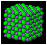
The total energy of LiH consists of three terms: the energy of the lithium cation, the energy of the hydride anion and the coulombic potential energy between the ions. As indicated below the cation‐anion potential energy depends on the relative size of ions.

\[ \begin{matrix} E_{cation} = \frac{9}{4R_c^2} - \frac{3Z_c}{R_c} + \frac{6}{5R_c} & E_{anion} = \frac{9}{4R_a^2} - \frac{3Z_a}{R_a} + \frac{6}{5R_a} \end{matrix} \nonumber \]

\[ \begin{matrix} \frac{R_c}{R_a} \geq 0.414 & E_{coul} = \frac{-1.748}{R_a + R_c} & \frac{R_c}{R_a} < 0.414 & E_{coul} = \frac{-1.748}{ \sqrt{2} R_a} \end{matrix} \nonumber \]

Nuclear charges: \( \begin{matrix} Z_a = 1 & Z_c = 3 \end{matrix}\)

Seed values for the ionic radii: \( \begin{matrix} R_a = .5 & R_c = .5 \end{matrix}\)

\[ \begin{array}{c|c} E_{LiH} \left( R_c,~R_a \right) = & \frac{9}{4R_c^2} - \frac{3Z_c}{R_c} + \frac{6}{5R_c} + \frac{9}{4R_a^2} - \frac{3Z_a}{R_a} + \frac{6}{5 R_a} - \frac{1.748}{R_a + R_c} ~ \text{if } \frac{R_c}{R_a} \geq 0.414 \\ ~ & \frac{9}{4R_c^2} - \frac{3Z_c}{R_c} + \frac{6}{5R_c} + \frac{9}{4R_a^2} - \frac{3Z_a}{R_a} + \frac{6}{5 R_a} - \frac{1.748}{R_a + R_c} ~ \text{otherwise} \end{array} \nonumber \]

\[ \begin{matrix} \begin{pmatrix} R_c \\ R_a \end{pmatrix} = \text{Minimize} \left( E_{LiH},~ R_c,~R_a \right) & \begin{pmatrix} R_c \\ R_a \end{pmatrix} = \begin{pmatrix} 0.577 \\ 1.482 \end{pmatrix} & E_{LiH} \left( R_c,~R_a \right) = -7.784 \end{matrix} \nonumber \]

Calculation of the energies of the gas-phase ions:

\[ \begin{matrix} E_c \left( R_c \right) = \frac{9}{4 R_c^2} - \frac{3Z_c}{R_c} + \frac{6}{5R_c} & R_c = \text{Minimize} \left( E_c,~R_c \right) & R_c = 0.577 & E_c \left( R_c \right) = -6.76 \\ E_c \left( R_c \right) = \frac{9}{4 R_a^2} - \frac{3Z_a}{R_a} + \frac{6}{5R_a} & R_a = \text{Minimize} \left( E_a,~R_a \right) & R_a = 2.500 & E_a \left( R_a \right) = -0.360 \end{matrix} \nonumber \]

Lattice energy calculation: LiH (s) --> Li⁺ (g) + H^- (g)

\[ E_c \left( R_c \right) + E_a \left( R_a \right) - E_{LiH} \left( R_c,~R_a \right) = 0.494 \nonumber \]

Li(s): Lithium metal is modeled as an ionic solid with the same face‐centered structure as used for LiH. The small spheres in the figure above are again the lithium cations and the large spheres are the electride anions, spherical electron charge clouds of radius Ra.

\[ \begin{array}{c|c} E_{LiH} \left( R_c,~R_a \right) = & \frac{9}{4R_c^2} - \frac{3Z_c}{R_c} + \frac{6}{5R_c} + \frac{9}{8R_a^2} - \frac{1.748}{R_a + R_c} ~ \text{if } \frac{R_c}{R_a} \geq 0.414 \\ ~ & \frac{9}{4R_c^2} - \frac{3Z_c}{R_c} + \frac{6}{5R_c} + \frac{9}{8R_a^2} - \frac{1.748}{ \sqrt{2} R_a} ~ \text{otherwise} \end{array} \nonumber \]

\[ \begin{matrix} \begin{pmatrix} R_c \\ R_a \end{pmatrix} = \text{Minimize} \left( E_{Li},~ R_c,~R_a \right) & \begin{pmatrix} R_c \\ R_a \end{pmatrix} = \begin{pmatrix} 0.577 \\ 1.82 \end{pmatrix} & E_{Li} \left( R_c,~R_a \right) = -7.1 \end{matrix} \nonumber \]

Lattice energy calculation for lithium metal assuming that the energy of a gas‐phase electron is zero: Li(s) ‐‐‐> Li⁺(g) + e^‐ (g)

\[ E_c \left( R_c \right) + 0 = E_{Li} \left( R_c,~R_a \right) = 0.34 \nonumber \]

Calculation of the enthalpy of formation of LiH(s) using the results of previous calculations: Li(s) + 1/2 H₂(g) ‐‐‐> LiH(s)

\[ -7.784 - \left( -7.1 - \frac{121}{2} \right) = -0.079 \nonumber \]

Methane: Two ionic models for methane are proposed in order to show that VSEPRʹs explanation for the greater stability of tetrahedral methane is spurious. Gillespieʹs Valence Shell Electron Pair Repulsion (VSEPR) theory [J. Chem. Educ. 40, 295 (1963)] holds that the configuration of valence electron pairs surrounding a central nonvalence nuclear kernel is determined by minimization of electron‐electron potential energy.

In the ionic models considered here the +4 carbon kernel (nucleus and nonvalence electrons) is treated as a point charge which interacts electrostatically with four unpolarized hydride anions of radius R in both the square planar (D4h) and tetrahedral (Td) arrangement. In Td methane the carbon kernel occupies the tetrahedral hole and is not visible in the figure below. The energy of the hydride anion as a function of charge cloud radius was calculated previously.

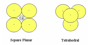
D4h: In the energy expression for square planar geometry the first term in brackets multiplied by four is the hydride ion energy contribution, the next two are the repulsive interactions between the hydrides and the final term is the attractive hydride‐kernel potential energy.

\[ E_{D4h} (R) = 4 \left( \frac{9}{4R^2} + \frac{6}{5R} - \frac{3}{R} \right) + \frac{2}{R} + \frac{1}{ \sqrt{2} R} - \frac{16}{ \sqrt{2} R} \nonumber \]

\[ \begin{matrix} R = R & \begin{array}{c|c} R = \frac{d}{dR} E_{D4h} (R) = 0 & _{ \text{float, 5}} ^{ \text{solve, R}} \rightarrow 1.1388 \end{array} & E_{D4h} (R) = -6.94 \end{matrix} \nonumber \]

\[ \begin{matrix} V_{hh} = \frac{2}{R} + \frac{1}{ \sqrt{2} R} = 2.377 & V_{hk} = - \frac{16}{ \sqrt{2} R} = -9.935 \end{matrix} \nonumber \]

Td: In the energy expression for tetrahedral geometry the repulsive interaction between the hydrides and the attractive hydride‐kernel potential energy follow the hydride ions energy contribution.

\[ E_{Td} (R) = 4 \left( \frac{9}{4R^2} + \frac{6}{5R} - \frac{3}{R} \right) - \frac{16}{ \sqrt{ \frac{3}{2}} R} \nonumber \]

\[ \begin{matrix} R = R & \begin{array}{c|c} R = \frac{d}{dR} E_{Td} (R) = 0 & _{ \text{float, 5}} ^{ \text{solve, R}} \rightarrow 1.0426 \end{array} & E_{Td} (R) = -8.279 \end{matrix} \nonumber \]

\[ \begin{matrix} V_{hh} = \frac{3}{R} = 2.877 & V_{hk} = - \frac{16}{ \sqrt{2} R} = -10.851 \end{matrix} \nonumber \]

These calculations show that indeed tetrahedral methane is the energetically preferred geometry and that the reason for this is the stronger hydride‐kernel attractive interaction, which is due to its smaller charge cloud radius and the close packing of the charge clouds around the nuclear kernel. The repulsive interaction between the hydride anions is actually higher in tetrahedral methane. In other words, molecular geometry is driven by maximizing the attractive electron‐nuclear interactions and not by minimizing the electron‐electron repulsive interactions.