
3.9: A Simple Charge Cloud Model for Molecular Hydrogen- Or, Is It a DFT Model?
- Page ID
- 152130

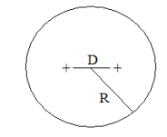
A simple charge cloud model for H2 is shown below (1,2). Two protons, separated by distance D, are symmetrically embedded in a uniform‐density, two‐electron spherical charge cloud of radius R.
In atomic units (h/2π = me = e = 4πε0 = 1) the total electronic energy based on this model is,
\[ E = \frac{9}{4R^2} - \frac{24}{5R} + \frac{D^2}{2R^3} + \frac{1}{D} \nonumber \]
The various energy components are identified below (3).
\[ \begin{matrix} \text{Electron kinetic energy:} & T = \frac{9}{4R^2} \\ \text{Electron-nucleus potential energy:} & V_{ne} = \frac{-6}{R} + \frac{D^2}{2R^3} \\ \text{Electron-electron potential energy:} & V_{ee} = \frac{6}{5R} \\ \text{Nucleus-nucleus potential energy:} & V_{nn} = \frac{1}{D} \end{matrix} \nonumber \]
The total electronic energy is minimized with respect to R for a series of internuclear separations, D, to generate an energy curve that can be used with the virial theorem to generate kinetic and potential energy contributions.
\[ \begin{matrix} \text{Seed values for the minimization algorithm:} & R = 1 & E = -2 \end{matrix} \nonumber \]
\[ \begin{matrix} \text{Given} & E = \frac{9}{4R^2} - \frac{24}{5R} + \frac{D^2}{2R^3} + \frac{1}{D} & \frac{d}{dR} \left( \frac{9}{4R^2} - \frac{24}{5R} + \frac{D^2}{2R^3} + \frac{1}{D} \right) = 0 & \text{E(D) = Find(R, E)} \end{matrix} \nonumber \]
Substitution of \( E(D) = T(D) + V(D)\) into the virial relation \(2T(D) + V(D) = -D \frac{d}{dD} E(D)\) yields expressions for the kinetic and potential energies given below.
\[ \begin{matrix} D = .1, .2 .. 6 & \text{Kinetic energy:} & T(D) = -E(D)_1 - D \frac{d}{dD} E(D)_1 \\ ~ & \text{Potential energy:} & V(D) = 2E(D)_1 + D \frac{d}{dD} E(D)_1 \end{matrix} \nonumber \]
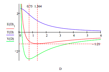
This graphic display of the total energy and its kinetic and potential energy components clearly shows that molecular stability depends on electron kinetic energy. The immediate cause of the total energy minimum is a rise in electron kinetic energy. In other words potential energy is still decreasing at D = 1.364, and doesnʹt start to rise sharply, due to electron and nuclear repulsion, until D = 0.75. So, although it is commonly thought and taught, electron and nuclear repulsion are not the immediate cause of atomic and molecular stability.
Minimization of the total energy simultaneously with respect to D and R locates the energy ground state and the equilibrium values of D and R precisely.
\[ \begin{matrix} \text{Seed values for the energy minimization:} & D = 1 & R = 3 \end{matrix} \nonumber \]
\[ \begin{matrix} E(R,~D) = \frac{9}{4R^2} - \frac{24}{5R} + \frac{D^2}{2R^3} + \frac{1}{D} & \begin{pmatrix} R \\ D \end{pmatrix} = \text{Minimize(E, R, D)} & \begin{pmatrix} R \\ D \end{pmatrix} = \begin{pmatrix} 1.364 \\ 1.364 \end{pmatrix} & \text{E(R, D) = -1.21} \end{matrix} \nonumber \]
Show that the virial theorem is obeyed:
\[ \left| \frac{V(R)}{T(D)} \right| = 2 \nonumber \]
The calculated internuclear separation, 1.364 a0, is in good agreement with the experimental bond length of 1.40 a0. However, the calculated ground state energy ‐1.21 Eh is lower than the experimental value ‐1.17 Eh. Thus in this calculation the virial theorem is satisfied, but the variational principle is violated.
It is the authorʹs opinion that the charge cloud approach is a primitive version of density functional theory (DFT), because as can be seen above, all energy components are calculated in terms of the electron density, the signature of the DFT method.
Literature cited:
- G. F. Neumark, Microfilm Abstr. 11, 834 (1951).
- L. M. Kleiss, Diss. Abstr. 14, 1562 (1954).
- F. Rioux, Am. J. Phys. 44, 56 (1976)