3.8: Two Analyses of the Covalent Bond using the Virial Theorem

Atomic and molecular stability and spectroscopy, and the nature of the chemical bond cannot be explained using classical physics: quantum mechanical principles are required. Bohr was a pioneer in an effort to apply an early version of quantum theory to these important issues with his models of the hydrogen atom and hydrogen molecule. Of course, Bohr's approach became "old" quantum mechanics and was abandoned in the 1920s with the creation of a "new" quantum mechanics by Heisenberg and Schrödinger and their collaborators. This tutorial deals exclusively with the chemical bond and summarizes Slater's contribution to our current understanding of the energetics of its formation using the virial theorem. Since the acceptance of the "new" quantum mechanics many others have contributed to the interpretation of chemical bond formation, but like Bohr, Slater was an insightful pioneer.

In a seminal paper, J. Chem. Phys. 1933, 1, 687-691, John C. Slater used the virial theorem to analyze chemical bond formation and was the first (in my opinion) to recognize the importance of kinetic energy in covalent bond formation. Regarding the universally valid virial theorem he wrote,

...this theorem gives a means of finding kinetic and potential energy separately for all configurations of the nuclei, as soon as the total energy is known, from experiment or theory.

The purpose of this tutorial is to demonstrate the validity of this assertion. The experimental method employs a Morse function for the energy of the hydrogen molecule ion parametrized using spectroscopic data. The theoretical approach is based on an ab initio LCAO-MO calculation of the energy based on a molecular orbital consisting a superposition of scaled hydrogen atomic orbitals.

Experimental Method

The kinetic energy, potential energy and total energy of the hydrogen molecule ion are calculated as a function of R using the virial theorem and a Morse function for the total energy based on experimental parameters.

Total energy:

\[ E(R) = T(R) + V(R) \nonumber \]

Virial theorem:

\[ 2T(R) + V(R) = -R \frac{d}{dR} E(R) \nonumber \]

Morse parameters:

\[ \begin{matrix} D_e = 0.103 E_h & R_e = 2.003 a_0 & \beta = 0.708 a_0^{-1} \end{matrix} \nonumber \]

These parameters are from Levine, I. N. Quantum Chemistry, 6^th ed., p. 400.

Morse function:

\[ E(R) = D_e \left[ 1 - \text{exp} \left[ - \beta \left( R - R_e \right) \right] \right]^2 - D_e \nonumber \]

Using equation (1) to eliminate V(R) in equation (2) yields an equation for kinetic energy as a function of the internuclear separation. Using equation (1) to eliminate T(R) in equation (2) yields an equation for potential energy as a function of the internuclear separation.

\[ T(R) - =E(R) - R \frac{d}{dR} E(R) \nonumber \]

\[ V(R) = 2E(R) + R \frac{d}{dR} E(R) \nonumber \]

These important equations determine the mean kinetic and potential energies as functions of R, one might almost say experimentally, directly from the curves of E as a function of R which can be found from band spectra. The theory is so simple and direct that one can accept the results without question....

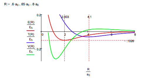
While the Morse calculation has an empirical flavor to it, its results are interpreted in terms of rudimentary quantum theory concepts. This energy profile shows that as the protons approach, the potential energy rises because molecular orbital formation (constructive interference) draws electron density away from the nuclei into the internuclear region. The kinetic energy decreases because molecular orbital formation brings about electron delocalization.

At about 4.1 a₀ this trend reverses as atomic orbital contraction begins. The kinetic energy rises because the volume occupied by the electron decreases and the potential energy decreases for the same reason: a smaller electronic volume brings the electron closer to the nuclei on average. Only at R ~ 1a₀ does nuclear repulsion cause the total potential energy to increase and contribute to the repulsion energy of the molecule. In other words, the kinetic energy increase is the immediate cause of the energy minimum or ground state.

Theoretical Method

The following LCAO-MO calculation uses a superposition of scaled 1s atomic orbitals and yields the following result for the energy of the hydrogen molecule ion as a function of the internuclear distance and the orbital scale factor.

\[ \begin{matrix} 1s_a = \sqrt{ \frac{ \alpha^3}{ \pi} \text{exp} ( - \alpha r_a )} & s_b = \sqrt{ \frac{ \alpha^3}{ \pi} \text{exp} ( - \alpha r_b )} & S_{ab} = \int 1s_a 1s_b d \tau & \Psi_{mo} = \frac{1s_a + 1s_b}{ \sqrt{2 + 2S_{ab}}} \end{matrix} \nonumber \]

\[ E ( \alpha,~R) = \frac{ - \alpha^2}{2} + \frac{ \left[ \alpha^2 - \alpha - \frac{1}{R} +\frac{1 + \alpha R}{R} \text{exp} (-2 \alpha R) + \alpha ( \alpha - 2) (1 + \alpha R) \text{exp} ( - \alpha R) \right]}{ \left[ 1 + \text{exp} \left( - \alpha,~R \right) \left( 1 + \alpha R + \frac{ \alpha^2 R^2}{3} \right) \right]} + \frac{1}{R} \nonumber \]

\[ \begin{matrix} \alpha = 1 & \text{Energy = -2} & \text{Given} & \text{Energy} = E( \alpha,~ R) & \frac{d}{d \alpha} E( \alpha,~R) = 0 & \text{Energy(R) = Find}( \alpha,~\text{Energy}) \end{matrix} \nonumber \]

As noted above, using \( E = T+V\) with the virial theorem \(2T + V = -R \frac{d}{dR}E\) leads to the following expressions for T and V.

\[ \begin{matrix} T(R) = - \text{Energy}(R)_1 -R \frac{d}{dR} \text{Energy}(R)_1 & V(R) = 2 \text{Energy}(R)_1 + R \frac{d}{dR} \text{Energy} (R)_1 & R = .2, .25 .. 10 \end{matrix} \nonumber \]

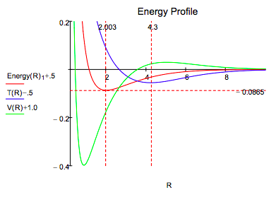
It is clear that both methods lead to very similar energy profiles. The only significant difference is that the Morse calculation leads to a lower energy minimum, -0.1026 Eh versus -0.0865 Eh for the molecular orbital calculation. Therefore, the interpretation provided for the Morse energy profile is valid for the LCAO-MO profile.

\[ \begin{matrix} \text{Conversion factors:} & a_o = 5.29177(10)^{-11} m & E_h = 4.359748(10)^{-18} \text{ joule} \end{matrix} \nonumber \]