
2.61: One-dimensional H-atom with Delta Function Potential
- Page ID
- 158676

The One‐dimensional Hydrogen Atom with a Delta Function Potential Energy Interaction Between the Proton and Electron
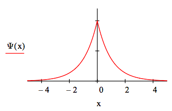
The energy Hamiltonian and a normalized wave function for the hydrogen atom with delta function interaction between the electron and proton is given below.
\[ \begin{matrix} \text{H} = - \frac{1}{2} \frac{d^2}{dx^2} \blacksquare - \Delta (x) \blacksquare & \Psi (x) = \text{exp} \left( - |x| \right) & \int_{- \infty}^{ \infty} \Psi (x)^2 dx \rightarrow 1 \end{matrix} \nonumber \]
The wave function is not well‐behaved in coordinate space making the evaluation of kinetic energy tricky. However, the evaluation of potential energy is straight forward. So the strategy is to evaluate potential energy in coordinate space and kinetic energy in momentum space. The latter requires a Fourier transform of the coordinate space wave function.
Calculation of Potential Energy in Coordinate Space
\[ V = \int_{- \infty}^{ \infty} \Psi (x) - \Delta (x) \Psi (x) \text{dx} \rightarrow - 1 \nonumber \]
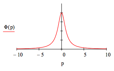
Fourier Transform of the Coordinate Wave Function into Momentum Space
\[ \Psi (p) = \int_{- \infty}^{ \infty} \frac{ \text{exp(-i p x)}}{ \sqrt{2 \pi}} \Psi (x) \text{dx simplify} \rightarrow \frac{ \sqrt{2}}{ \sqrt{ \pi} \left( p^2 + 1 \right)} \nonumber \]
Display the Momentum Wave Function to Show it is Well-behaved
Calculation of Kinetic Energy in Momentum Space
\[ \text{T} = \int_{- \infty}^{ \infty} \Phi (p) \frac{p^2}{2} \Phi (p) \text{dp simplify} \rightarrow \frac{1}{2} \nonumber \]
Calculation of Total Energy
\[ \text{E = T + V} \rightarrow \text{E} = - \frac{1}{2} \nonumber \]
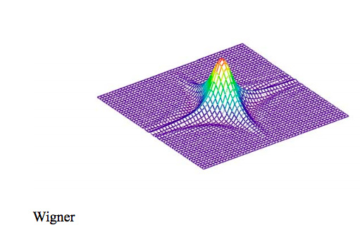
The Wigner Function
The Wigner phase‐space distribution function is calculated using the momentum wave function.
\[ \text{W(x, p)} = \frac{1}{2 \pi} \int{- \infty}^{ \infty} \overline{ \Phi \left( \text{p} + \frac{ \text{s}}{2} \right)} \text{exp(-i s x)} \Phi \left( \text{p} - \frac{ \text{s}}{2} \right) \text{ds} \nonumber \]
\[ \begin{matrix} N = 50 & i = 0 .. N & x_i = -4 + \frac{8i}{N} & j = 0 .. N & p_j = -7 + \frac{14j}{N} & \text{Wigner}_{i,~j} = \text{W} \left( x_i,~ p_j \right) \end{matrix} \nonumber \]
Next we look at two variational calculations on the same system. The first involves a gaussian trial wave function, and the second a trigonmetric trial wave function.
Gaussian Trial Wave Function
\[ \begin{matrix} \Psi_1 (x,~ \beta ) = \left( \frac{2 \beta}{ \pi} \right)^{ \frac{1}{4}} \text{exp}\left( - \beta x^2 \right) & \int_{- \infty}^{ \infty} \Psi_1 (x,~ \beta)^2 \text{dx assume, } \beta >0 \rightarrow 1 \end{matrix} \nonumber \]
Evaluation of Variational Energy Integral
\[ \text{E} ( \beta ) = \int_{- \infty}^{ \infty} \Psi_1 (x,~ \beta ) - \frac{1}{2} \frac{d^2}{dx^2} \Psi (x,~ \beta ) \text{dx... assume, } \beta > 0 \rightarrow \frac{ \beta}{2} - \frac{ \sqrt{2} \sqrt{3}}{ \sqrt{ \pi}} + \int_{- \infty}^{ \infty} - \Delta (x) \Psi_1 (x,~ \beta)^2 dx \nonumber \]
Energy Minimization With Respect to Variational Parameter
\[ \begin{matrix} \frac{d}{d \beta} \text{E} ( \beta = 0 \text{ solve, } \beta \rightarrow \frac{2}{ \pi} & \begin{array}{c|c} \text{E} ( \beta ) & _{ \text{simplify}}^{ \text{substitute, } \beta = \frac{2}{ \pi}} \rightarrow - \frac{1}{ \pi} = -0.318 \end{array} \end{matrix} \nonumber \]
Error
\[ \left| \frac{-.318+ .5}{-.5} \right| = 36.4 \% \nonumber \]
Trigonometric Trial Wave Function
\[ \begin{matrix} \Psi_2 ( \text{x}, ~ \beta ) = \sqrt{ \frac{ \beta}{2}} \text{sech} ( \beta \text{x} ) & \end{matrix} \nonumber \]
Evaluation of Variational Energy Integral
\[ \begin{matrix} \text{E} ( \beta ) = \begin{array}{c|c} \int_{ - \infty}^{ \infty} \Psi_2 ( \text{x},~ \beta ) - \frac{1}{2} \frac{d^2}{dx^2} \Psi_2 ( \text{x, } \beta ) dx ... & _{ \text{simplify}}^{ \text{assume, } \beta > 0} \rightarrow \frac{ \beta ( \beta -3}{6} \\ + \int_{ - \infty}^{ \infty} - \Delta ( \text{x}) \Psi_2 ( \text{x, } \beta )^2 dx \end{array} \end{matrix} \nonumber \]
Energy Minimization With Respect to Variational Parameter
\[ \begin{matrix} \frac{d}{d \beta} \text{E} ( \beta ) = 0 \text{ solve, } \beta \rightarrow \frac{3}{2} & \begin{array}{c|c} \text{E} ( \beta ) & _{ \text{simplify}}^{ \text{substitute, } \beta = \frac{3}{2}} \rightarrow - \frac{3}{8} = -0.375 \end{array} \end{matrix} \nonumber \]
Error
\[ \left| \frac{-.375 + .5}{-.5} \right| = 25 \% \nonumber \]
Graphical Comparison of Exact Wave Function with Trial Wave Function
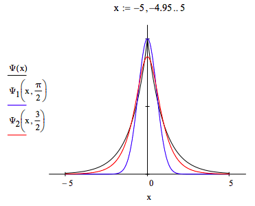
This graphical comparison is consistent with the variational results presented above. The trigonometric trial function more closely resembles the exact wave function.