2.29: A Bohr Model for Multi-electron Atoms and Ions

Abstract

A deBroglie Bohr model is described that can be used to calculate the electronic energies of atoms or ions containing up to four electrons. Seven exercises are provided which can be used to give students training in doing energy audits, carrying out simple variational calculations and critically analyzing the calculated results.

This note builds on two publications in the pedagogical literature [1,2] that showed how extending the Bohr model to two‐ and three‐electron atoms and ions could be used to enhance student understanding of atomic structure. A Bohr model, more correctly a deBroglie‐Bohr model, is used here to calculate the total electronic energies of atoms and ions containing up to four electrons.

The Bohr model for the hydrogen atom is the prototype of the semi‐classical approach to atomic and molecular structure. Although it was superseded by quantum mechanics many decades ago, it is still taught today because of its simplicity and because it introduced several important quantum mechanical concepts that have survived the model: quantum number, quantized energy, and quantum jump.

When applied to multi‐electron atoms and ions, the Bohr model provides a pedagogical tool for improving studentsʹ analytical and critical skills. As will be demonstrated, given a ʺpictureʺ of an atom or ion, it is not unrealistic to expect an undergraduate student to identify all the contributions to the total electronic energy, carry out an energy minimization and interpret the results in a variety of ways. Seven student exercises, with answers, are provided to illustrate how this might be accomplished.

We begin with a review of the deBroglie‐Bohr model for the hydrogen atom. Working in atomic units (h = 2π, m_e = e = 4πε₀ = 1), and using the deBroglie‐Bohr restriction on electron orbits (nλ =2πR_n, where n = 1, 2, 3, ...), the deBroglie wave equation (λ = h/mv) and Coulombʹs law the total electron energy is the following sum of its kinetic and potential energy contributions.

\[ E_n = \frac{n^2}{2R_n^2} - \frac{1}{R_n} \nonumber \]

Minimization of the energy with respect to the variational parameter Rn yields the allowed orbit radii and energies.

\[ \begin{matrix} R_n = n^2 a_0 \\ E_n = \frac{-0.5E_h}{n^2} \end{matrix} \nonumber \]

where a₀ = 52.9 pm and Eh = 4.36 x 10^‐18 joule.

The model shown in the figure below is for the beryllium atom or any four‐electron ion. Note that the occupancy of the inner orbit is restricted to two electrons (Pauli Principle) and that the orbit radii are constrained by the hydrogen atom result (R₂ = 4R₁) leaving only one variational parameter, the radius of the n = 1 orbit.

With these model elements and a little geometry [2] it is easy to specify the kinetic and potential energy contributions to the total energy. The numeric subscripts refer to the quantum number of the orbit. Thus T₁ is the kinetic energy of an electron in the n = 1 orbit, V_N1 is the potential energy interaction of an electron in the n = 1 orbit with the nucleus, and V₁₂ is the potential energy interaction of an electron in the n = 1 orbit with an electron in the n = 2 orbit.

The recommended student calculations described below are carried out in the Mathcad programming environment [3]. A Mathcad file for doing the exercises is available for download on the Internet [4]. The calculation for the beryllium atom is carried out as shown below. Required student input is indicated by the highlighted regions.

Enter nuclear charge: Z = 4

Kinetic energy:

\[ \begin{matrix} T_1 \left( R_1 \right) = \frac{1}{2 R_1^2} & T_2 \left( R_1 \right) = \frac{1}{8 R_1^2} \end{matrix} \nonumber \]

Electron-nucleus potential energy:

\[ \begin{matrix} V_{N1} \left( R_1 \right) = \frac{-Z}{R_1} & V_{N2} \left( R_1 \right) = \frac{-Z}{4 R_1} \end{matrix} \nonumber \]

Electron-electron potential energy:

\[ \begin{matrix} V_{11} \left( R_1 \right) = \frac{1}{2R_1} & V_{22} \left( R_1 \right) = \frac{1}{8 R_1} & V_{12} \left( R_1 \right) = \frac{1}{ \sqrt{17} R_1} \end{matrix} \nonumber \]

The next step is to do an energy audit for the atom or ion under consideration. The student is prompted to weight each of the contributions to the total electronic energy. The entries given below are appropriate for the Bohr beryllium atom shown in the figure above.

Enter coefficients for each contribution to the the total energy:

\[ \begin{matrix} T_1 \left( R_1 \right) & T_2 \left( R_1 \right) & V_{N1} \left( R_1 \right) & V_{N2} \left( R_1 \right) & V_{11} \left( R_1 \right) & V_{22} \left( R_1 \right) & V_{12} \left( R_1 \right) \\ \colorbox{yellow}{a = 2} & \colorbox{yellow}{b = 2} & \colorbox{yellow}{c = 2} & \colorbox{yellow}{d = 2} & \colorbox{yellow}{e = 1} & \colorbox{yellow}{f = 1} & \colorbox{yellow}{g = 4} \end{matrix} \nonumber \]

The energy of the Bohr atom/ion in terms of the variational parameter R1, the radius of the inner electron orbit, and the various kinetic and potential energy contributions is:

\[ E \left( R_1 \right) = a T_1 \left( R_1 \right) + b T_2 \left( R_1 \right) + c V_{N1} \left( R_1 \right) + d V_{N2} \left( R_1 \right) + e V_{11} \left( R_1 \right) + f V_{22} \left( R_1 \right) + g V_{12} \left( R_1 \right) \nonumber \]

Minimization of the electronic energy of the Bohr atom/ion with respect to R1 yields the optimum inner orbit radius and ground‐state energy

\[ \begin{matrix} \begin{array}{c|c} R_1 = \frac{d}{dR_1} E \left( R_1 \right) = 0 & _{ \text{float, 5}}^{ \text{solve, R}_1} \rightarrow .29744 \end{array} & E \left( R_1 \right) = -14.128 \end{matrix} \nonumber \]

Thus, this model predicts a stable beryllium atom with an electronic energy in error by less than 4%. However, it must be stressed that the main purpose of the exercises presented is not to promote the Bohr model as such, but to use it as a vehicle for providing students with training in doing energy audits, carrying out simple variational calculations and critically analyzing the calculated results.

In the student exercises critical analysis will involve assessing the level of agreement with experimental results, and whether or not the variational principle and the virial theorem are satisfied. Because the second exercise involves the virial theorem as criterion for validity, it is recommended that the first and second exercises be done in tandem.

Student Exercises

Exercise 1: Use this worksheet to calculate the ground state energy for H, He, Li and Be, and confirm all the entries in the table below. The experimental ground state energy of an atom is the negative of the sum of the successive ionization energies given in the data table in the Appendix A.

\[ \begin{pmatrix} \text{Element} & \frac{ \text{E(calc)}}{E_h} & \frac{ \text{E(exp)}}{E_h} & \% \text{Error} \\ \text{H} & -0.500 & -0.500 & 0 \\ \text{He} & -3.062 & -2.904 & 5.46 \\ \text{Li} & -7.385 & -7.480 & 1.26 \\ \text{Be} & -14.128 & -14.672 & 3.71 \end{pmatrix} \nonumber \]

This assignment shows that, given its simplicity, the Bohr model achieves acceptable results. However, the students should note that the He result violates the variational theorem. In other words, the calculated energy is lower than the experimental energy.

Exercise 2: An important criterion for the validity of a quantum mechanical calculation is satisfying the virial theorem which for atoms and ions requires: E = ‐T = V/2. Demonstrate whether or not the virial theorem is satisfied for the elements in the first exercise.

Calculate the kinetic energy:

\[ \begin{matrix} T \left( R_1 \right) = a T_1 \left( R_1 \right) + b T_2 \left( R_1 \right) & T \left( R_1 \right) = 14.129 \end{matrix} \nonumber \]

Calculate potential energy:

\[ \begin{matrix} V \left( R_1 \right) = E \left( R_1 \right) - T \left( R_1 \right) & V \left( R_1 \right) = -28.257 & \frac{V \left( R_1 \right)}{2} = -14.129 \end{matrix} \nonumber \]

\[ \begin{matrix} \text{Element} & \frac{ \text{E(calc)}}{E_h} & \frac{ \text{ -T(calc)}}{2E_h} & \text{VTSatisfied} \\ \text{H} & -0.500 & -0.500 & -0.500 & \text{Yes} \\ \text{He} & -3.062 & -3.062 & -3.062 & \text{Yes} \\ \text{Li} & -7.385 & -7.385 & -7.385 & \text{Yes} \\ \text{Be} & -14.128 & -14.129 & -14.129 & \text{Yes} \end{matrix} \nonumber \]

The Bohr model satisfies the virial theorem for all atomic calculations (atoms and ions). This does not guarantee the validity of the model. However, any model calculation that violates the virial theorem indicates that the model is not quantum mechanically valid.

Exercise 3: Plot the total energy, and the kinetic and potential energy components on the same graph for beryllium and interpret the results.

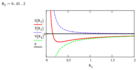
This graph clearly shows that atomic stability is the result of two competing energy terms. The attractive coulombic potential energy interaction draws the electrons toward the nucleus. At large R₁ values this term dominates and the electron orbits gets smaller. However, this attractive interaction is overcome at small R₁ values by the ʺrepulsiveʺ character of kinetic energy term that dominates at small R₁ values and an energy minimum, a ground‐state is achieved.

Exercise 4: Calculate the ground state energies of some cations (He⁺, Li⁺, Be⁺, B⁺, C²⁺) and compare your calculations with experimental results using the data table in Appendix A.

\[ \begin{pmatrix} \text{Cation} & \frac{ \text{E(calc)}}{E_h} & \frac{ \text{E(exp)}}{E_h} & \% \text{Error} \\ \text{He}^1 & -2.000 & -2.000 & 0 \\ \text{Li}^1 & -7.562 & -7.282 & 3.70 \\ \text{Be}^1 & -14.275 & -14.329 & 0.38 \\ \text{B}^1 & -23.782 & -24.348 & 2.33 \\ \text{C}^2 & -35.938 & -36.613 & 1.88 \end{pmatrix} \nonumber \]

Just as in the first exercise, the one‐electron species He+1 is in exact agreement with experiment and the two‐electron ion, Li⁺, violates the variational theorem.

Exercise 5: Use the results of exercises 1 and 3 to calculate the first ionization energies of H, He, Li and Be and compare your results with the experimental data available in Appendix A.

\[ \begin{pmatrix} \text{Element} & \frac{ \text{E(atom)}}{E_h} & \frac{ \text{E(ion)}}{E_h} & \frac{ \text{IE(calc)}}{E_h} & \frac{ \text{IE(exp)}}{E_h} \\ \text{H} & -0.500 & 0 & 0.500 & 0.500 \\ \text{He} & -3.063 & -2.000 & 1.063 & 0.904 \\ \text{Li} & -7.385 & -7.562 & -0.177 & 0.198 \\ \text{Be} & -14.128 & -14.275 & -0.147 & 0.343 \end{pmatrix} \nonumber \]

The results for H and He are acceptable, but both Li and Be have negative ionization energies.

Exercise 6: Are the anions of H, He and Li stable? In other words, do they have energies lower than the neutral species?

\[ \begin{pmatrix} \text{Anion} & \frac{ \text{Eion(calc)}}{E_h} & \frac{ \text{Eatom(exp)}}{E_h} & \text{Stable} \\ \text{H}^{-1} & -0.562 & -0.500 & \text{Yes} & \text{He}^{-1} & -2.745 & -2.904 & \text{No} \\ \text{Li}^{-1} & -6.681 & -7.480 & \text{No} \end{pmatrix} \nonumber \]

The Bohr model gets these results correct. However, it should be noted that Li‐1 is stable in liquid ammonia.

Exercise 7: Do a two‐parameter variational calculation on the beryllium atom shown in the Figure. In other words, minimize the total electronic energy of a beryllium atom that has two electrons in an orbit of radius R₁ and two electrons in another orbit of radius R₂.

As outlined in Appendix B this calculation yields the following results: R₁ = R₂ = 0.329 a₀ and E(R₁, R₂) = ‐18.518 E_h, an energy significantly lower than calculated for beryllium in Exercise 1. Thus, in the absence of the orbital occupancy restriction of the exclusion principle, energy minimization places all electrons in the ground state orbit. It was a realization of this that lead Pauli in part to formulate the exclusion principle.

In summary, the purpose of this note is to use the Bohr model as an initial vehicle to help students develop skill in carrying out basic atomic structure calculations and to critically analyze the results of those calculations.

Appendix A

Data: Successive Ionization Energies for the First Six Elements

\[ \begin{pmatrix} \text{Element} & \text{IE}_1& \text{IE}_2 & \text{IE}_3 & \text{IE}_4 & \text{IE}_5 & \text{IE}_6 \\ \text{H} & 0.500 & x & x & x & x & x \\ \text{He} & 0.904 & 2.000 & x & x & x & x \\ \text{Li} & 0.198 & 2.782 & 4.500 & x & x & x \\ \text{Be} & 0.343 & 0.670 & 5.659 & 8.000 & x & x \\ \text{B} & 0.305 & 0.926 & 1.395 & 9.527 & 12.500 & x \\ \text{C} & 0.414 & 0.896 & 1.761 & 2.370 & 14.482 & 18.000 \end{pmatrix} \nonumber \]

Appendix B

Energy contributions for the two‐parameter Bohr calculation:

\[ \begin{matrix} T_1 \left( R_1 \right) = \frac{1}{2R_1^2} & T_2 \left( R_2 \right) = \frac{1}{2 R_2^2} & V_{N1} \left( R_1 \right) = \frac{-Z}{R_1} & V_{N2} \left( R_2 \right) = \frac{-Z}{R_2} \\ V_{11} \left( R_1 \right) = \frac{1}{2R_1} & V_{22} \left( R_2 \right) = \frac{1}{2 R_2} & V_{12} \left( R_1,~R_2 \right) = \frac{1}{ \sqrt{R_1^2 + R_2^2}} \end{matrix} \nonumber \]

\[ E \left( R_1,~R_2 \right) = 2 T_1 \left( R_1 \right) + 2 T_2 \left( R_2 \right) + 2 V_{N1} \left( R_1 \right) + 2 V_{N2} \left( R_2 \right) + V_{11} \left( R_1 \right) + V_{22} \left( R_2 \right) + 4 V_{12} \left( R_1,~R_2 \right) \nonumber \]

Minimization of the electronic energy with respect to R₁ and R₂:

\[ \begin{matrix} \begin{pmatrix} R_1 \\ R_2 \end{pmatrix} = \begin{pmatrix} 1 \\ 4 \end{pmatrix} & \begin{pmatrix} R_1 \\ R_2 \end{pmatrix} = \text{Minimize} \left( E,~ R_1,~R_2 \right) & \begin{pmatrix} R_1 \\ R_2 \end{pmatrix} = \begin{pmatrix} 0.329 \\ 0.329 \end{pmatrix} & \text{E} \left( R_1,~ R_2 \right) = -18.518 \end{matrix} \nonumber \]

Literature cited:

1. Bagchi, B.; Holody, P. ʺAn interesting application of Bohr theory,ʺ Am. J. Phys. 1988, 56, 746.
2. Saleh‐Jahromi, A. ʺGround State Energy of Lithium and Lithium‐like Atoms Using the Bohr Theory,ʺ The Chemical Educator, 2006, 11, 333‐334.
3. Mathcad is a product of Mathsoft, 101 Main Street, Cambridge, MA 02142
4. www.users.csbsju.edu/~frioux/stability/BohrAtoms.mcd