10.33: Variational Method for the Feshbach Potential

Last updated
Save as PDF

Page ID: 136983

\( \newcommand{\vecs}[1]{\overset { \scriptstyle \rightharpoonup} {\mathbf{#1}} } \) \( \newcommand{\vecd}[1]{\overset{-\!-\!\rightharpoonup}{\vphantom{a}\smash {#1}}} \)\(\newcommand{\id}{\mathrm{id}}\) \( \newcommand{\Span}{\mathrm{span}}\) \( \newcommand{\kernel}{\mathrm{null}\,}\) \( \newcommand{\range}{\mathrm{range}\,}\) \( \newcommand{\RealPart}{\mathrm{Re}}\) \( \newcommand{\ImaginaryPart}{\mathrm{Im}}\) \( \newcommand{\Argument}{\mathrm{Arg}}\) \( \newcommand{\norm}[1]{\| #1 \|}\) \( \newcommand{\inner}[2]{\langle #1, #2 \rangle}\) \( \newcommand{\Span}{\mathrm{span}}\) \(\newcommand{\id}{\mathrm{id}}\) \( \newcommand{\Span}{\mathrm{span}}\) \( \newcommand{\kernel}{\mathrm{null}\,}\) \( \newcommand{\range}{\mathrm{range}\,}\) \( \newcommand{\RealPart}{\mathrm{Re}}\) \( \newcommand{\ImaginaryPart}{\mathrm{Im}}\) \( \newcommand{\Argument}{\mathrm{Arg}}\) \( \newcommand{\norm}[1]{\| #1 \|}\) \( \newcommand{\inner}[2]{\langle #1, #2 \rangle}\) \( \newcommand{\Span}{\mathrm{span}}\)\(\newcommand{\AA}{\unicode[.8,0]{x212B}}\)

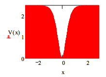
Define potential energy: V₀ = 2.5 d = 0.5 \(V(x) = V_o \tanh \left( \dfrac{x}{d}\right)^2\)

Display potential energy:

Screen Shot 2019-02-15 at 12.00.50 PM.png

Choose Gaussian trial wavefunction:

\[ \psi (x, \beta ) = \left( \frac{2 \beta}{ \pi} \right) ^{ \frac{1}{4}} exp ( - \beta x^2) \nonumber \]

Demonstrate that the trial wavefunction is normalized.

\[ \int_{- \infty}^{ \infty} \psi (x, \beta )^2 dx~~~assume,~ \beta > 0 \rightarrow 1 \nonumber \]

Evaluate the variational integral.

\[ E( \beta ) = \int_{ - \infty}^{ \infty} \psi (x, \beta ) \frac{-1}{2} \frac{d^2}{dx^2} \psi (x, \beta ) dx + \int_{- \infty}^{ \infty} V(x) \psi (x, \beta )^2 dx \nonumber \]

Minimize the energy integral with respect to the variational parameter, \( \beta\).

\( \beta\) = 1 \( \beta\) = Minimize (E, \( \beta\)) \( \beta\) = 0.913 E( \( \beta\)) = 1.484

Calculate the % error given that numerical integration of Schrödingerʹs equation (see next tutorial) yields E = 1.44949 E_h.

\[ \frac{E( \beta ) - 1.44949}{1.44949} \times 100 = 2.36 \nonumber \]

Display wavefunction in the potential well.

Screen Shot 2019-02-15 at 12.05.40 PM.png

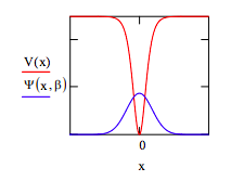
Calculate the probability that tunneling is occurring.

\[ V(x) = 1.484 |_{float,~3}^{solve,~x} \rightarrow {\begin{pmatrix} -1.511 \\ 0 .511 \end{pmatrix}} \nonumber \]

\[ 2 \int_{0.511}^{ \infty} \psi (x, \beta )^2 dx = 0.329 \nonumber \]