
Variational Method
- Page ID
- 64918
The Variational Method is a mathematical method that is used to approximately calculate the energy levels of difficult quantum systems. It can also be used to approximate the energies of a solvable system and then obtain the accuracy of the method by comparing the known and approximated energies. The Schrödinger equation can be solved exactly for our model systems including Particle in a Box (PIB), Harmonic Oscillator (HO), Rigid Rotor (RR), and the Hydrogen Atom. However, for systems that have more than one electron, the Schrödinger equation cannot be analytically solved and requires approximation like the variational method to be used.
The Schrödinger equation takes the form:
\[\hat{H} \psi = E \psi \label{schro}\]
with the Hamiltonian operator \(\hat{H}\) representing the sum of kinetic energy (\(T\)) and potential energy (\(V\)):
\[\hat {H} = T + V\]
For the helium atom, the Hamiltonian can be expanded to the following:
\[\hat{H} = -\dfrac{\hbar^2}{2m_e}\bigtriangledown_{el_{1}}^2 -\dfrac{\hbar^2}{2m_e}\bigtriangledown_{el_{2}}^2 - \dfrac {Ze^2}{4\pi\epsilon_0 r_1} - \dfrac {Ze^2}{4\pi\epsilon_0 r_2} + \dfrac {e^2}{4\pi \epsilon_0 r_{12}}\label{8}\]
where
- \(r_1\) and \(r_2\) are distances of electron 1 and electron 2 from the nucleus
- \(r_{12}\) is the distance between the two electrons (\(r_{12})= | r_1 - r_2|\)
- \(Z\) is the charge of the nucleus (2 for helium)
Solving the Schrödinger equation for helium is impossible to solve because of the electron-electron repulsion term in the potential energy:
\[\dfrac {e^2}{4\pi\epsilon_0 r_{12}}\]
Because of this, approximation methods were developed to be able to estimate energies and wavefunctions for complex systems. The variational method is one such approxation and perturbation theory is another.
Because of a chemist's dependence on said approximation methods, it is very important to understand the accuracy of these methods. This can be done by applying the method to simple known systems.
The variational method is useful because of its claim that the energy calculated for the system is always more than the actual energy.
\[ E_{\phi} \ge E_o \]
It does this by introducing a trial wavefunction and then calculating the energy based on it. If the trial wavefunction is chosen correctly, the variational method is quite accurate. If the trial wavefunction is poor, the energy calculated will not be very accurate, but it will always be larger than the true value. The greater than or equal symbol is used because if by chance the trial wavefunction that is guessed is the actual wavefunction that describes a system, then the trial energy is equal to the true energy.
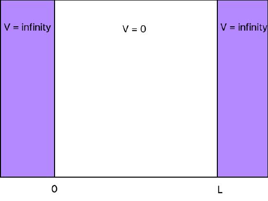
When trying to find the energy of a particle in a box, set the boundaries at x = 0 and x = L as shown in the diagram below.
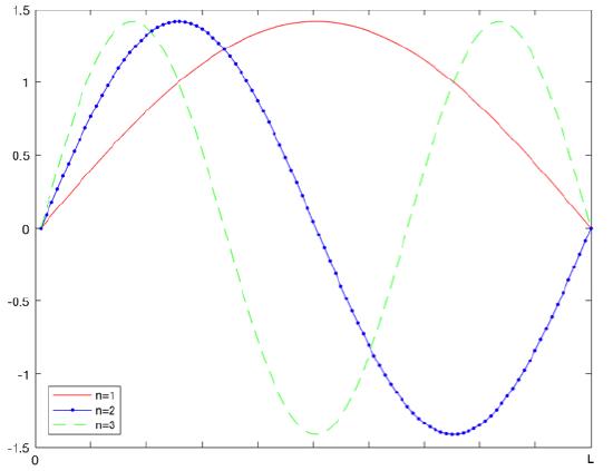
The true solution of the Schrödinger equation is well known as:
\[\psi _{n}(x)=\sqrt{\dfrac{2}{L}} sin \dfrac{n\pi x}{L} \]
With the energy levels being:
\[E_{n}=\dfrac{\hbar^2\pi^2}{2mL^2}\, n^2=\dfrac{h^2}{8mL^2}n^2\; \; \; \; n=1,2,,3...\]
The following describes the variational method equation that is used to find the energy of the system. H is the Hamiltonian operator for the system.
How to choose a Trial Wavefunction?
- The trial function must have the characteristics that classify it as a wavefunction, ie. continuous, etc.
- The trial function need to have the same general shape as the true wavefunction.
- The trial function must have the same boundary conditions.
- To improve accuracy, the trial wavefunction can be represented as linear combinations of single trial wavefunctions.
Variational Theorem
\[E_{trial} = \dfrac{\langle \phi_{trial}| \hat{H} | \phi_{trial} \rangle }{\langle \phi_{trial}| \phi_{trial} \rangle} \label{theorem}\]
The denominator above is only necessary if the trial wavefunction needs to normalized.
- When given a trial wavefunction, sometimes the problem states if it is normalized or not.
- When forced to decide, if there is a constant in front of the function, that is usually assumed to be the normalization constant. If a constant is not present then there is no normalization constant and the denominator in Equation \ref{theorem} is necessary.
Picking a trial wavefunction for particle in a box
A trial function for the \(n=1\) system is:
\[\phi_{trial} = x(L-x)\]
where this function is not normalized. Is this a good guess for the system? To find out we must apply the variational theorem to find the energy.
\[E_{trial} = \dfrac{\langle \phi_{trial}| \hat{H} | \phi_{trial} \rangle }{\langle \phi_{trial}| \phi_{trial} \rangle}\]
For PIB we know our Hamiltonian is \(\dfrac{-\hbar^2}{2m}\dfrac{d^2}{dx^2}\)
\[E_{trial} = \dfrac{\langle \phi_{trial}| \dfrac{-\hbar^2}{2m}\dfrac{d^2}{dx^2} | \phi_{trial} \rangle }{\langle \phi_{trial}| \phi_{trial} \rangle}\]
By putting in our trial \(\phi\), our trial energy becomes:
\[E_{trial} = \dfrac{\langle Nx(L-x)| \dfrac{-\hbar^2}{2m}\dfrac{d^2}{dx^2} |Nx(L-x)\rangle}{\langle Nx(L-x)|Nx(L-x)\rangle}\]
Solve the numerator:
Then we calculate the numerator of \((1)\):
\[\langle\varphi | H | \varphi\rangle = \int_{0}^{L}x(L−x) (- \dfrac{\hbar^2}{2m}\dfrac{d^2}{dx^2}) x(L−x)dx = \\- \dfrac{\hbar^2}{2m} \int_{0}^{L} (xL - x^2) (-2) dx = \dfrac{\hbar^2}{m} (L\dfrac{x^2}{2} - \dfrac{x^3}{3}) \Biggr\rvert_{0}^{L} = \dfrac{\hbar^2}{m} (\dfrac{L^3}{2} - \dfrac{L^3}{3}) = \dfrac{\hbar^2}{m} \dfrac{L^3(3-2)}{6} = \dfrac{\hbar^2 L^3}{6m} \]
Find the denominator:
\[\langle x(L-x)|x(L-x)\rangle = N^2\]
\[N^2 = \langle (xL-x^2)(xL-x^2)\rangle = langle x^2L^2-x^3L-x^3L+x^4\rangle = \int_{0}^{L} x^2L^2-2x^3L+x^4 dx = \dfrac{L^5}{3}-\dfrac{L^5}{2}+\dfrac{L^5}{5} = \dfrac{L^5}{30}\]
\[N = \sqrt{\dfrac{L^5}{30}}\]
Now put them together
\[\dfrac{\langle\varphi| H | \varphi\rangle}{\langle\varphi |\varphi\rangle} = \dfrac{30}{L^5} \dfrac{\hbar^2 L^3}{6m} = \dfrac{5\hbar^2}{mL^2}\]
The conclusion is:
\[E_1 \leq \dfrac{5\hbar^2}{mL^2}\]
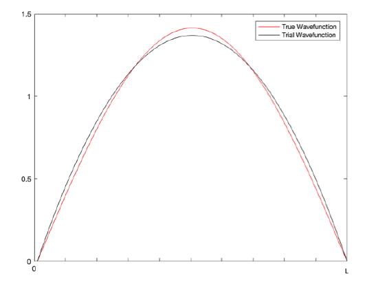
As seen in the diagram above, the trial wavefunction follows the shape of the true wavefunction and has the same boundary conditions, so it is a good guess for the system.
A Different Trial Wavefunction: Linear Combination of Wavefunctions
The accuracy of the variational method can be greatly enhanced by the use of a trial function with additional terms. We can try this out by repeating the earlier steps with the following wavefunction:
\[\phi_{trial} = x(L-x)+Cx^2(L-x)\]
The normalization constant was omitted because it is not necessary to find the energy. \(C\) in this equation is a variational parameter. When inserting this equation into our variational theorem and then into a programming application we yield:
\[E_{trial} = \dfrac{\int_{0}^{L} \phi_{trial}(\dfrac{-\hbar^2}{2m}\dfrac{d^2}{dx^2}\phi_{trial})dx}{\int_{0}^{L} \phi_{trial}\phi_{trial} dx} = \dfrac{\dfrac{1}{105}C^2+\dfrac{1}{15}C+\dfrac{1}{6}}{\dfrac{1}{630}C^2+\dfrac{1}{70}C+\dfrac{1}{30}}\]
Because the trial energy is always larger than the actual energy, we can minimize the trial energy by taking the derivative with respect to C, setting it equal to zero and solving for C. The smaller energy when plugging in all found values of C is the closest to the true energy.
\[\dfrac{d}{dC}(E_{trial}) = \dfrac{\dfrac{1}{105}C^2+\dfrac{1}{15}C+\dfrac{1}{6}}{\dfrac{1}{630}C^2+\dfrac{1}{70}C+\dfrac{1}{30}}-\dfrac{\dfrac{1}{105}C^2+\dfrac{1}{15}C+\dfrac{1}{6}}{(\dfrac{1}{630}C^2+\dfrac{1}{70}C+\dfrac{1}{30})^2}\dfrac{1}{315}C+\dfrac{1}{70}\]
\[0=3\dfrac{4C^2+14C-21}{(C^2+9C+21)^2}\]
\[C = -\dfrac{7}{4}+\dfrac{1}{4}\sqrt{133} ; -\dfrac{7}{4}-\dfrac{1}{4}\sqrt{133}\]
Plugging in we get a smaller value when using the first term for \(C\) and we get that
\[E_{trial} = 4.9348748\] \[\%error = 0.0015\%\]
This error is much smaller than that of our first wavefunction, which shows that a linear combination of terms can be more accurate than one term by itself and describe the system much better. It is actually necessary to use this method of guessing for the wavefunction for excited states of a system. If we were to do the same for the first excited state of the particle in a box, then the percent error would go from 6.37% error to 0.059% error. This shows how crucial this method of linearly combining terms to form trial wavefunctions becomes with the excited states of systems. Without this method the excited states would not be nearly as accurate as needed.
The Variational Theorem states that the trial energy can be only greater or equal to the true energy (Equation \ref{theorem}). But when does the Variational Method give us the exact energy that we are looking for?
Let's use the Harmonic Oscillator as our system.
\[\phi_{trial} = e^{-\alpha x^2}\]
\[V = \dfrac{1}{2} kx^2\]
\[ T = -\dfrac{\hbar^2}{2m}\dfrac{d^2}{dx^2}\]
First find the denominator:
\[\langle \phi_{trial}|\phi_{trial}\rangle\]
\[\int_{-\infty}^{\infty} dx(e^{-\alpha x^2})*(e^{-\alpha x^2}) = \int_{-\infty}^{\infty}(e^{-2\alpha x^2})dx\]
\[\langle \phi_{trial}|\phi_{trial}\rangle = \sqrt{\dfrac{\pi}{2\alpha}}\]
Then find the numerator:
\[\langle\varphi | H | \varphi\rangle = \langle\varphi | T | \varphi\rangle +\langle\varphi | V | \varphi\rangle\]
\[ = \dfrac{1}{2k}\dfrac{1}{4\alpha}\sqrt{\dfrac{\pi}{2\alpha}}\dfrac{\hbar^2 \alpha}{2m}\]
\[E_{\phi} = \dfrac{k}{8 \alpha} +\dfrac{\hbar^2 \alpha}{2m}\]
Now because there is a variational constant, \(\alpha\) we need to minimize it
\[\dfrac{dE_{\phi}}{d\alpha} = -\dfrac{k}{8\alpha^2}+\dfrac{\hbar^2}{2m} = 0\]
\[ \alpha = \dfrac{\sqrt{km}}{2\hbar}\]
Now we plug this into the \(E_{\phi}\) for \(\alpha\) and we will find \(E_{\phi min}\)
\[E_{\phi min} = \dfrac{\hbar}{4} \sqrt{\dfrac{k}{m}} + \dfrac{\hbar}{4} \sqrt{\dfrac{k}{m}}\]
Where \(w = \sqrt{\dfrac{k}{m}}\)
\[E_{\phi min} = \dfrac{1}{2} \hbar w\]
Now we can plug in our minimum \(\alpha\) into our \(\phi_{trial}\) and we need to introduce our normalization constant.
\[\phi_{\alpha min} = (\dfrac{2\alpha}{\pi})^{\dfrac{1}{4}} e^{-\dfrac{\sqrt{km}x^2}{2\hbar}}\]
If you notice, this is the exact equation for the Harmonic Oscillator ground state. We were able to find this by initially guessing a good wave function, and varying and minimizing the variational constant.
For a more in depth step by step video on this example: Click here
Linear Variational Method
Another approximation method that is used to study molecules is the linear variational method. It includes having a trial wavefunction with a linear combination of \(n\) linearly independent functions of f. More information can be found here.
References
- Youtube, TMP Chem, www.youtube.com/watch?v=-Df6...LM&spfreload=5
- W. Tandy Grubbs, Department of Chemistry, Unit 8271, Stetson University, DeLand, FL 32720 (wgrubbs@stetson.edu), www.chemeddl.org/alfresco/ser...pdf?guest=true
Contributors and Attributions
- Ashleigh Falasco