
3.2.2: Pre-equilibrium Approximation
- Page ID
- 1411
The pre-equilibrium approximation assumes that the reactants and intermediates of a multi-step reaction exist in dynamic equilibrium.
Introduction
According to the steady state approximation article, reactions involving many steps can be analyzed using approximations. Like the steady state method, the pre-equilibrium approximation method derives an expression for the rate of product formation with approximated concentrations. Unlike the steady state method, the pre-equilibrium approximation does so by assuming that the reactants and intermediate are in equilibrium. Although both methods are used to solve for a rate of reaction, they are used under different conditions. The steady state method can only be used if the first step of a reaction is much slower than the second step, whereas the pre-equilibrium approximation requires the first step to be faster. These opposing conditions prevent the two methods from being interchangeable.
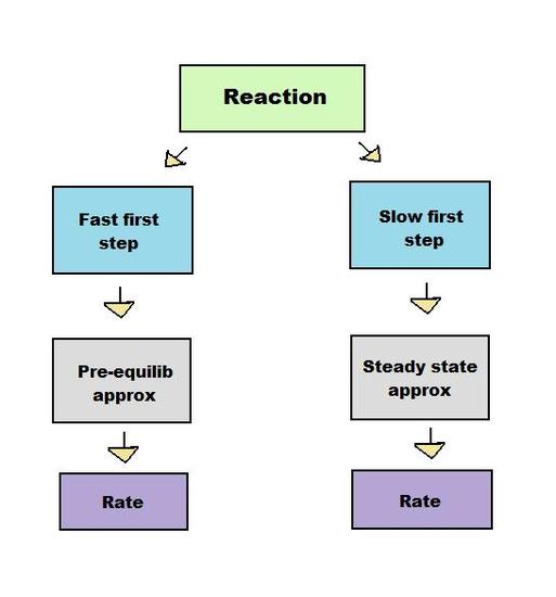
Both the steady state approximation and pre-equilibrium approximation apply to intermediate-forming consecutive reactions, in which the product of the first step of the reaction serves as the reactant for the second step.
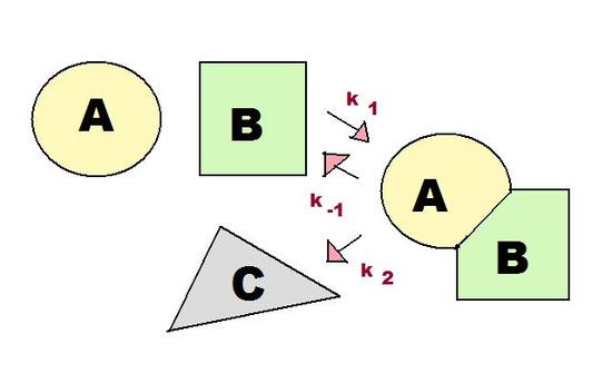
As shown in Figure 1, there are three rate constants in the consecutive reaction involving an intermediate. These three rate constants, k1, k-1, and k2, are incredibly important for the pre-equilibrium approximation, as discussed in the next section.
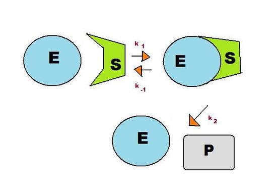
A consecutive reaction found in living systems is the enzyme-substrate reaction. In this type of reaction, an enzyme binds to a substrate to produce an enzyme-substrate intermediate, which then forms the final product. As shown in Figure 2, this reaction follows the basic pattern of the consecutive reaction in Figure 1. The two reactants, E (enzyme) and S (substrate), form the intermediate ES. This enzyme-substrate intermediate forms the product P, usually an essential biomolecule. The enzyme then exits the reaction unchanged and able to catalyze future reactions.
As before, there are three reaction rates in this reaction: k1, k-1, and k2. The pre-equilibrium approximation uses the rate constants to solve for the rate of the reaction, indicating how quickly the reaction is likely to produce the biomolecule.
Derivation of the Rate Law
The enzyme substrate reaction in Figure 2 is used below to demonstrate a rate law derivation. The overall strategy for the pre-equilibrium reaction is as follows:
I. Assume reactants and intermediate are in equilibrium
- Write out the general reaction
- Break the overall reaction into elementary steps
- Assume the reactants and the intermediate are in equilibrium throughout the reaction
II. Solve for the rate of product formation
- Write out the rate of product formation using the equilibrium constant, K
- Simplify this rate by incorporating the composite rate constant
- Simplify to as few variables as possible
I. Assume Reactants and Intermediate are in Equilibrium
1. The general reaction used to derive a rate law is as following:
\( E + S \xrightleftharpoons[k_{-1}]{\ k_1\ } ES \xrightarrow{k_2} E + P \)
2. Breaking up the overall reaction into elementary steps gives:
\[E + S \rightarrow ES \nonumber \] Rate of formation of ES = k1 [E][S]
\[ES \rightarrow E + S \nonumber \] Rate of decay of ES = k-1 [ES]
\[ES \rightarrow E + P \nonumber \] Rate of formation of P = k2 [ES]
3. In the steady state reaction, the intermediate concentration [ES] is assumed to remain at a small constant value. The pre-equilibrium approximation takes a different approach. Because the reversible reaction \(E + S \rightarrow ES\) is much faster than the product formation of \(ES \rightarrow E + P\), E, S, and ES are considered to be in equilibrium throughout the reaction. This concept greatly simplifies the mathematics leading to the rate law.
II. Solve for the Rate of Product Formation
4. Using the idea that the reactants and intermediate are in equilibrium, the rate of formation of E + P can be written as:
\[\frac{d[P]}{dt}=k_2[ES]=k_2K[E][S] \nonumber \]
where
\[K = \frac{[ES]}{[E][S]} = \frac{k_1}{k_{-1}} \nonumber \]
5. The rate of product formation is simplified through the composite rate constant, k:
6. The rate of product formation can now be shortened to:
\[\dfrac{d[P]}{dt} = k[E][S] \nonumber \]
This equation can be solved for unknown variables in consecutive reactions involving intermediates.
Activation Energies in the Pre-equilibrium Reaction
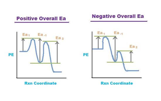
Figure 4. Potential Energy (PE) vs Rxn Coordinate for two pre-equilibrium reactions.
Left graph shows a positive overall activation energy (Ea > 0) and right graph shows a
negative overall activation energy (Ea < 0).
Many reactions have at least one activation energy that must be reached in order for the reaction to go forward. There are three activation energies in a pre-equilibrium reaction: two for the reversible steps and one for the final step. The three activation energies are denoted Ea,1 Ea,-1, and Ea,2:
| Ea,1 |
Forward |
| Ea,-1 |
Reverse |
| Ea,2 |
Product Formation |
The overall activation energy is given below:
The overall activation energy is positive if Ea1 + Ea2> Ea-1 The overall activation energy is negative if Ea1 + Ea2 < Ea -1
Practice Problem
For the reaction \(A + B \xrightarrow[k_{-1}]{k_1} AB \xrightarrow[]{k_2} C\)(see Figure 1), derive a rate law using the pre-equilibrium approximation.
Solution
\(\dfrac{d[P]}{dt} = k[A][B]\) where \(k =\dfrac{k_1 k_2}{k_{-1}}\)
Outside Links
- Discussion of both pre-equilibrium and steady state approximations with Java applet figures: www.ch.cam.ac.uk/magnus
- Supplemental material on pre-equilibrium approximation (zoom in for better view): www.chem.yorku.ca/profs/bohme/notes/II3P11.gif
- An example of the pre-equilibrium approximation being used in current research (see equation 10 in Results and Discussion): http://www.biochemj.org/bj/373/0337/bj3730337.htm
References
- Atkins, Peter, and de Paula, Julio. Physical Chemistry for the Life Sciences. New York, NY: W. H. Freeman and Company, 2006. Pages 275-276.
- Chang, Raymond. Physical Chemistry for the Biosciences. Sausalito, CA: University Science Books, 2005. Pages 368-369.
Contributors and Attributions
- Tamara Kadir