2.2: Continuous Probability Theory

Probability Density

Although the outcomes of measurements can be discretized, and in fact, are invariably discretized when storing the data, in theory it is convenient to work with continuous variables where physical quantities are assumed to be continuous. For instance, spatial coordinates in phase space are assumed to be continuous, as are the momentum coordinates for translational motion in free space.

To work with continuous variables, we assume that an event can return a real number instead of an integer index. The real number with its associated probability density \(\rho\) is a continuous random number. Note the change from assigning a probability to an event to assigning a probability density. This is necessary as real numbers are not countable and thus the number of possible events is infinite. If we want to infer a probability in the usual sense, we need to specify an interval \([l,u]\) between a lower bound \(l\) and an upper bound \(u\). The probability that trial \(\mathcal{T}\) will turn up a real number in this closed interval is given by

\[P([l,u]) = \int_l^u \rho(x) \mathrm{d}x \ .\]

The probability density must be normalized,

\[\int_{-\infty}^{\infty} \rho(x) \mathrm{d} x = 1 \ .\]

A probability density distribution can be characterized by its moments.

The \(n^\mathrm{th}\) moment of a probability density distribution is defined as,

\[\begin{align} & \langle x^n \rangle = \int_{-\infty}^\infty x^n \rho(x) \mathrm{d}x \ .\end{align}\]

The first moment is the mean of the distribution. With the mean \(\langle x \rangle\), the central moments are defined

\[\begin{align} & \langle (x-\langle x \rangle)^n \rangle = \int_{-\infty}^\infty (x-\langle x \rangle)^n \rho(x) \mathrm{d}x \ .\end{align}\]

The second central moment is the variance \(\sigma_x^2\) and its square root \(\sigma_x\) is the standard deviation. [concept:moment_analysis]

Probability density is defined along some dimension \(x\), corresponding to some physical quantity. The average of a function \(F(x)\) of this quantity is given by

\[\langle F(x) \rangle = \int_{-\infty}^\infty F(x) \rho(x) \mathrm{d}x \ .\]

In many books and articles, the same symbol \(P\) is used for probabilities and probability densities. This is pointed out by Swendsen who decided to do the same, pointing out that the reader must learn to deal with this. In the next section he goes on to confuse marginal and conditional probability densities with probabilities himself. In these lecture notes we use \(P\) for probabilities, which are always unitless, finite numbers in the interval \([0,1]\) and \(\rho\) for probability densities, which are always infinitesimally small and may have a unit. Students are advised to keep the two concepts apart, which means using different symbols.

Figure \(\PageIndex{1}\): Generation of random numbers that conform to a given probability density distribution. (A) Cumulative probability distribution \(P(x) = \int_{-\infty}^x \rho(\xi) \mathrm{d} \xi\) for \(\rho(x) = \exp(-x^4)\) (blue). A pseudo-random number with uniform distribution in \((0,1)\), here 0.75, selects the ordinate of \(P(x)\) (red dashed horizontal line). The corresponding abscissa, here \(x = 0.45\) (red dashed vertical line), is an instance of a random number with probability density distribution \(\rho(x)\). (B) Distribution of \(10^5\) random numbers (grey line) and target probability density distribution \(\rho(x) = \exp(-x^4)\) (black line).

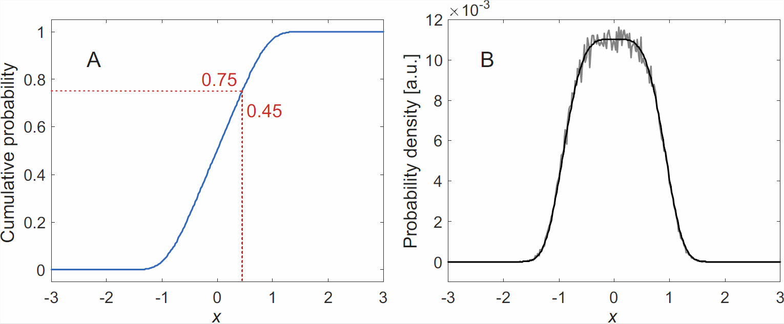
Computer representations of probability densities by a vector or array are discretized. Hence, the individual values are finite. We now consider the problem of generating a stream of random numbers that conforms to a given discretized probability density \(\vec{\rho}\). Modern programming languages or mathematical libraries include functions that provide uniformly distributed pseudo-random numbers in the interval \((0,1)\) (Matlab: rand) or pseudo-random numbers with a Gaussian (normal) distribution with mean 0 and standard deviation 1 (Matlab: randn). A stream of uniformly distributed pseudo-random numbers in \((0,1)\) can be transformed to a stream of numbers with probability density conforming to \(\vec{\rho}\) by selecting for each input number the abscissa where the cumulative sum of \(\vec{\rho}\) (Matlab: cumsum(rho)) most closely matches the input number (Figure \(\PageIndex{1}\)). Note that \(\vec{\rho}\) must be normalized (Matlab: rho = rho/sum(rho)). Since a random number generator is usually called very often in a Monte Carlo simulation, the cumulative sum cumsum_rho should be computed once for all before the loop over all trials. With this, generation of the abscissa index poi becomes a one-liner in Matlab: [~,poi] = min(abs(cumsum_rho - rand));⁷

Coming back to physical theory, the concept of probability density can be extended to multiple dimensions, for instance to the \(2F = 2fM\) dimensions of phase space. Probability then becomes a volume integral in this hyperspace. A simple example of a multidimensional continuous problem is the probability of finding a classical particle in a box. The probability to find it at a given point is infinitely small, as there are infinitely many of such points. The probability density is uniform, since all points are equally likely for a classical (unlike a quantum) particle. With the volume \(V\) of the box, this uniform probability density is \(1/V\) if we have a single particle in the box. This follows from the normalization condition, which is \(\int \rho \mathrm{d}V = 1\). Note that a probability density has a unit, in our example m\(^{-3}\). In general, the unit is the inverse of the product of the units of all dimensions.

The marginal probability density for a subset of the events is obtained by ’integrating out’ the other events. Let us assume a particle in a two-dimensional box with dimensions \(x\) and \(y\) and ask about the probability density along \(x\). It is given by

\[\rho_x(x) = \int_{-\infty}^\infty \rho(x,y) \mathrm{d}y \ .\]

Likewise, the conditional probability density \(\rho(y|x)\) is defined at all points where \(\rho_x(x) \neq 0\),

\[\rho(y|x) = \frac{\rho(x,y)}{\rho_x(x)} \ .\]

If two continuous random numbers are independent, their joint probability density is the product of the two individual probability densities,

\[\rho(x,y) = \rho_x(x) \rho_y(y) \ .\]

Figure \(\PageIndex{2}\): Monte Carlo simulation of a two-dimensional probability density distribution. (A) Two-dimensional probability density distribution corresponding to the first-order membrane function used in the Matlab logo. (B) Distribution of \(10^7\) random numbers conforming to the probability density distribution shown in (A).

Exercise \(\PageIndex{1}\)

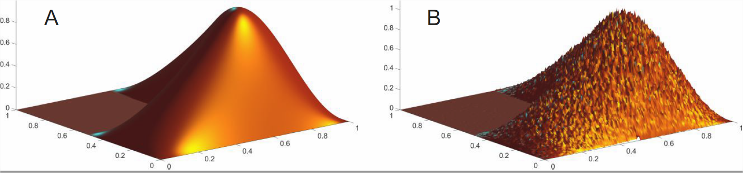
Write a Matlab program that generates random numbers conforming to a two-dimensional probability density distribution \(\rho_\mathrm{mem}\) that resembles the Matlab logo (Figure \(\PageIndex{2}\)). The (not yet normalized) distribution \(\rho_\mathrm{mem}\) is obtained with the function call L = membrane(1,resolution,9,9);. Hint: You can use the reshape function to generate a vector from a two-dimensional array as well as for reshaping a vector into a two-dimensional array. That way the two-dimensional problem (or, in general, a multi-dimensional problem) can be reduced to the problem of a one-dimensional probability density distribution.

Selective Integration of Probability Densities

We already know how to compute probability from probability density for a simply connected parameter range. Such a range can be an interval \([l,u]\) for a probability density depending on only one parameter \(x\) or a simply connected volume element for a probability density depending on multiple parameters. In a general problem, the points that contribute to the probability of interest may not be simply connected. If we can find a function \(g(x)\) that is zero at the points that should contribute, we can solve this problem with the Dirac delta function, which is the continuous equivalent of the Kronecker delta that was introduced above.

Concept \(\PageIndex{1}\): Dirac delta function

The Dirac delta function is a generalized function with the following properties

1. The function \(\delta(x)\) is zero everywhere except at \(x=0\).
2. \(\int_{-\infty}^\infty \delta(x) \mathrm{d}x = 1\).

The function can be used to select the value \(f(x_0)\) of another continuous function \(f(x)\),

\[\begin{align} & f(x_0) = \int_{-\infty}^\infty f(x) \delta(x-x_0) \mathrm{d}x \ .\end{align}\]

This concept can be used, for example, to compute the probability density of a new random variable \(s\) that is a function of two given random variables \(x\) and \(y\) with given joint probability density \(\rho(x,y)\). The probability density \(\rho(s)\) corresponding to \(s = f(x,y)\) is given by

\[\rho(s) = \int_{-\infty}^\infty \int_{-\infty}^\infty \rho(x,y) \delta\left( s - f(x,y) \right) \mathrm{d} x \mathrm{d} y \ .\]

Note that the probability density \(\rho(s)\) computed that way is automatically normalized.

Figure \(\PageIndex{3}\): Probability density distributions for two continuous random numbers \(x\) and \(y\) that are uniformly distributed in the interval \([0,6]\) and have zero probability density outside this interval. a) Marginal probability density \(\rho_x(x)\). b) Marginal probability density \(\rho_y(y)\). c) Joint probability density \(\rho(x,y)\). In the light blue area, \(\rho = 1/36\), outside \(\rho = 0\). The orange line corresponds to \(s = 4\) and the green line to \(s = 8\).

We now use the concept of selective integration to compute the probability density \(\rho(s)\) for the sum \(s = x+y\) of the numbers shown by two continuous dice, with each of them having a uniform probability density in the interval \([0,6]\) (Figure \(\PageIndex{3}\)). We have

\[\begin{align} \rho(s) & = \int_{-\infty}^\infty \int_{-\infty}^\infty \rho(x,y) \delta\left( s -(x+y) \right) \mathrm{d} y \mathrm{d} x \\ & = \frac{1}{36} \int_0^6 \int_0^6 \delta\left( s -(x+y) \right) \mathrm{d} y \mathrm{d} x \ .\end{align}\]

The argument of the delta function in the inner integral over \(y\) can be zero only for \(0 \leq s-x \leq 6\), since otherwise no value of \(y\) exists that leads to \(s = x+y\). It follows that \(x \leq s\) and \(x \geq s-6\). For \(s=4\) (orange line in Fig. [fig:cont_sum]c) the former condition sets the upper limit of the integration. Obviously, this is true for any \(s\) with \(0 \leq s \leq 6\). For \(s = 8\) (orange line in Fig. [fig:cont_sum]c) the condition \(x \geq s-6\) sets the lower limit of the integration, as is also true for any \(s\) with \(6 \leq s \leq 12\). The lower limit is 0 for \(0 \leq s \leq 6\) and the upper limit is 6 for \(6 \leq s \leq 12\). Hence,

\[\rho(s) = \frac{1}{36} \int_0^s \mathrm{d} s = \frac{s}{36} \ \mathrm{for} \ s \leq 6 \ ,\]

and

\[\rho(s) = \frac{1}{36} \int_{s-6}^6 \mathrm{d} s = \frac{12-s}{36} \ \mathrm{for} \ s \geq 6 \ .\]

From the graphical representation in Fig. [fig:cont_sum]c it is clear that \(\rho(s)\) is zero at \(s = 0\) and \(s = 12\), assumes a maximum of \(1/6\) at \(s = 6\), increases linearly between \(s=0\) and \(s=6\) and decreases linearly between \(s=6\) and \(s=12\).