2.37: Hund's Rule - Singlet-Triplet Calculations with Mathcad

Two-parameter Study of the 1s2s Excited State of He and Li⁺ - Hund's Rule

The trial variational wave functions for the 1s¹2s¹ excited state of helium atom and lithium ion are scaled hydrogen 1s and 2s orbitals:

\[ \begin{matrix} \Psi_{1s} ( r,~ \alpha ) = \sqrt{ \frac{ \alpha^3}{ \pi}} \text{exp} ( - \alpha r) & \Psi_{2s} (r,~ \beta ) = \sqrt{ \frac{ \beta^3}{32 \pi}} (2 - \beta r ) \text{exp} \left( \frac{- \beta r}{2} \right) \end{matrix} \nonumber \]

Nuclear charge: Z = 3

Seed values for α and β: \( \begin{matrix} \alpha = Z + 1 & \beta = Z - 1 \end{matrix}\)

The purpose of this analysis is to illustrate Hund's rule by calculating the energy of the singlet and triplet states for the 1s¹2s¹ electronic configuration. The singlet state has a symmetric orbital wave function and the triplet state has an antisymmetric orbital wave function:

\[ \begin{matrix} \Psi_S = \frac{1s(1)2s(2)+1s(2)2s(1)}{ \sqrt{2 + 2S_{1s2s}^2}} & \Psi_T = \frac{1s(1)2s(2)-1s(2)2s(1)}{ \sqrt{2 - 2S_{1s2s}^2}} \end{matrix} \nonumber \]

The integrals required for variational calculations on these states are given below:

\[ \begin{matrix} T_{1s} ( \alpha ) = \frac{ \alpha^2}{2} & T_{2s} ( \beta ) = \frac{ \beta^2}{8} & V_{N1s} ( \alpha ) = - Z \alpha & V_{N2s} ( \beta ) = \frac{-Z \beta}{4} \end{matrix} \nonumber \]

\[ \begin{matrix} T_{1s2s} ( \alpha,~ \beta ) = -4 \sqrt{2 \alpha^5 \beta^5} \frac{ \beta - 4 \alpha}{( \beta + 2 \alpha )^4} & V_{N1s2s} ( \alpha,~ \beta ) = 4 Z \sqrt{2 \alpha^3 \beta^3} \frac{-2 \alpha + \beta}{( \beta + 2 \alpha)^3} \\ V_{1212} ( \alpha,~ \beta ) = 16 \alpha^3 \beta^3 \frac{13 \beta^2 + 20 \alpha^2 - 30 \beta \alpha}{( \beta + 2 \alpha)^7} & S_{1s2s} ( \alpha,~ \beta) = 32 \sqrt{2 \alpha^3 \beta^3} \frac{ \alpha - \beta}{( \beta + 2 \alpha)^4} \\ V_{1122} ( \alpha,~ \beta ) = \beta \alpha \frac{ \beta^4 + 10 \beta^3 \alpha + 8 \alpha^4 + 20 \alpha^3 \beta + 12 \beta^2 \alpha^2}{( \beta + 2 \alpha)^5} \end{matrix} \nonumber \]

The next step in this calculation is to collect these terms in an expression for the energy of the singlet and triplet states and then minimize the energy with respect to the variational parameters, α and β. The results of this minimization procedure are shown below.

Singlet state calculation:

\[ E_S ( \alpha,~ \beta ) = \begin{array} T_{1s} ( \alpha ) + T_{2s} ( \beta ) + 2 T_{1s2s} ( \alpha,~ \beta ) S_{1s2s} ( \alpha,~ \beta ) ... \\ + V_{N1s} ( \alpha ) + V_{N2s} ( \beta ) + 2 V_{N1s2s} ( \alpha,~ \beta ) S_{1s2s} ( \alpha,~ \beta ) ... \\ + V_{1122} ( \alpha,~ \beta ) + V_{1212} ( \alpha,~ \beta ) \\ \hline 1 + S_{1s2s} ( \alpha,~ \beta)^2 \end{array} \nonumber \]

\[ \begin{matrix} \begin{pmatrix} \alpha \\ \beta \end{pmatrix} = \text{Minimize} \left( E_s,~ \alpha,~ \beta \right) & \begin{pmatrix} \alpha \\ \beta \end{pmatrix} = \begin{pmatrix} 3.019 \\ 1.681 \end{pmatrix} \end{matrix} \nonumber \]

Break down the total energy into kinetic, electron-nuclear potential, and electron-electron potential energy.

\[ \begin{matrix} T = \begin{array}{c} T_{1s} ( \alpha ) + T_{2s} ( \beta ) ... \\ + 2 T_{1s2s} ( \alpha,~ \beta ) S_{1s2s} ( \alpha,~ \beta ) \\ \hline 1 + S_{1s2s} ( \alpha,~ \beta )^2 \end{array} & V_{ne} = \begin{array}{c} V_{N1s} ( \alpha ) + V_{N2s} ( \beta ) ... \\ + 2 V_{N1s2s} ( \alpha,~ \beta ) S_{1s2s} ( \alpha,~ \beta ) \\ \hline 1 + S_{1s2s} ( \alpha,~ \beta )^2 \end{array} & V_{ee} = \begin{array}{c} V_{1122} ( \alpha, ~ \beta ) + V_{1212} ( \alpha,~ \beta ) \\ \hline 1 + S_{1s2s} ( \alpha,~ \beta )^2 \end{array} \end{matrix} \nonumber \]

\[ \begin{matrix} T = 5.091 & V_{ne} = -10.629 & V_{ee} = 0.448 & E_s ( \alpha,~ \beta ) = -5.091 \end{matrix} \nonumber \]

Calculate <r_1s>, <r_2s> and the absolute magnitude of the 1s-2s overlap:

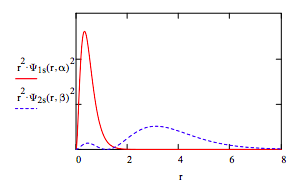
\[ \begin{matrix} \int_0^{ \infty} r \Psi_{1s} (r,~ \alpha)^2 4 \pi r^2 dr = 0.497 & \int_0^{ \infty} r \Psi_{2s} (r,~ \beta )^2 4 \pi r^2 dr = 3.569 & \int_0^{ \infty} \left| \Psi_{1s} (r,~ \alpha ) \Psi_{2s} (r,~ \beta ) \right| 4 \pi r^2 dr = 0.251 \end{matrix} \nonumber \]

Display the radial distribution function for the 1s and 2s orbitals:

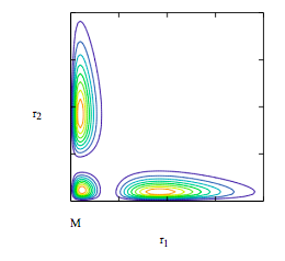
Display contour plot of singlet wave function:

\[ \begin{matrix} i = 0 .. 80 & r1_i = .085i & j = 0 .. 80 & r2_j = .085 j \end{matrix} \nonumber \]

\[ \begin{matrix} \Psi (r1,~ r2 ) = \frac{ \Psi_{1s} (r1,~ \alpha ) \Psi_{2s} (r2,~ \beta ) + \Psi_{1s} (r2,~ \alpha ) \Psi_{2s} (r1,~ \beta)}{ \sqrt{2 \left( 1 + S_{1s2s} ( \alpha,~ \beta )^2 \right)}} r1 r2 & M_{i,~ j} = \Psi \left( r1_i,~ r2_j \right)^2 \end{matrix} \nonumber \]

Triplet state calculation:

\[ E_S ( \alpha,~ \beta ) = \begin{array} T_{1s} ( \alpha ) + T_{2s} ( \beta ) - 2 T_{1s2s} ( \alpha,~ \beta ) S_{1s2s} ( \alpha,~ \beta ) ... \\ + V_{N1s} ( \alpha ) + V_{N2s} ( \beta ) + 2 V_{N1s2s} ( \alpha,~ \beta ) S_{1s2s} ( \alpha,~ \beta ) ... \\ + V_{1122} ( \alpha,~ \beta ) - V_{1212} ( \alpha,~ \beta ) \\ \hline 1 - S_{1s2s} ( \alpha,~ \beta)^2 \end{array} \nonumber \]

Minimization of E(α, β) simultaneously with respect to α and β. \( \begin{matrix} \alpha = Z & \beta = Z - 1 \end{matrix}\)

\[ \begin{matrix} \begin{pmatrix} \alpha \\ \beta \end{pmatrix} = \text{Minimize} \left( E_T,~ \alpha,~ \beta \right) & \begin{pmatrix} \alpha \\ \beta \end{pmatrix} = \begin{pmatrix} 2.999 \\ 2.570 \end{pmatrix} \end{matrix} \nonumber \]

Break down the total energy into kinetic, electron-nuclear potential, and electron-electron potential energy.

\[ \begin{matrix} T = \begin{array}{c} T_{1s} ( \alpha ) + T_{2s} ( \beta ) ... \\ + -2 T_{1s2s} ( \alpha,~ \beta ) S_{1s2s} ( \alpha,~ \beta ) \\ \hline 1 - S_{1s2s} ( \alpha,~ \beta )^2 \end{array} & V_{ne} = \begin{array}{c} V_{N1s} ( \alpha ) + V_{N2s} ( \beta ) ... \\ + -2 V_{N1s2s} ( \alpha,~ \beta ) S_{1s2s} ( \alpha,~ \beta ) \\ \hline 1 - S_{1s2s} ( \alpha,~ \beta )^2 \end{array} & V_{ee} = \begin{array}{c} V_{1122} ( \alpha, ~ \beta ) + V_{1212} ( \alpha,~ \beta ) \\ \hline 1 - S_{1s2s} ( \alpha,~ \beta )^2 \end{array} \end{matrix} \nonumber \]

\[ \begin{matrix} T = 5.103 & V_{ne} = -10.684 & V_{ee} = 0.479 & E_T ( \alpha,~ \beta ) = -5.103 \end{matrix} \nonumber \]

Calculate <r_1s>, <r_2s> and the absolute magnitude of the 1s-2s overlap:

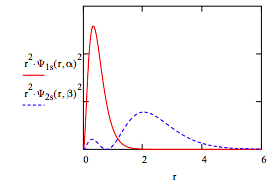
\[ \begin{matrix} \int_0^{ \infty} r \Psi_{1s} (r,~ \alpha )^2 4 \pi r^2 dr = 0.500 & \int_0^{ \infty} r \Psi_{2s} (r,~ \beta )^2 4 \pi r^2 dr = 2.334 & \int_0^{ \infty} \left| \Psi_{1s} (r,~ \alpha ) \Psi_{2s} (r,~ \beta ) \right| 4 \pi r^2 dr = 0.328 \end{matrix} \nonumber \]

Display the radial distribution function for the 1s and 2s orbitals:

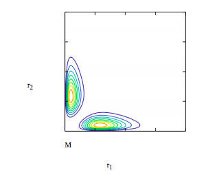
Display contour plot of singlet wave function:

\[ \begin{matrix} \Psi (r1,~ r2 ) = \frac{ \Psi_{1s} (r1,~ \alpha ) \Psi_{2s} (r2,~ \beta ) - \Psi_{1s} (r2,~ \alpha ) \Psi_{2s} (r1,~ \beta)}{ \sqrt{2 \left( 1 - S_{1s2s} ( \alpha,~ \beta )^2 \right)}} r1 r2 & M_{i,~ j} = \Psi \left( r1_i,~ r2_j \right)^2 \end{matrix} \nonumber \]

Summary of the calculations for the helium atom and lithium ion:

\[ \begin{pmatrix} \text{HundsRule} & \text{Helium} & \text{o} & \text{Atom} & \text{Lithium} & \text{o} & \text{Ion} \\ \text{Property} & \text{Singlet} & \Delta & \text{Triplet} & \text{Singlet} & \Delta & \text{Triplet} \\ \alpha & 2.013 & -0.019 & 1.994 & 3.019 & -0.020 & 2.999 \\ \beta & 0.925 & 0.626 & 1.551 & 1.681 & 0.889 & 2.570 \\ E & -2.170 & 0.003 & -2.167 & -5.091 & -0.012 & -5.103 \\ V_{ne} & -4.594 & -0.026 & -4.260 & -10.629 & -0.055 & -10.684 \\ V_{ee} & 0.254 & 0.033 & 0.287 & 0.448 & 0.031 & 0.479 \\ r_{1s} & 0.745 & 0.007 & 0.752 & 0.497 & 0.003 & 0.500 \\ r_{2s} & 6.489 & -2.620 & 3.869 & 3.569 & -1.235 & 2.334 \\ \int | 1s2s | d \tau & 0.232 & 0.072 & 0.304 & 0.251 & 0.077 & 0.328 \end{pmatrix} \nonumber \]

• The triplet state has a lower energy than the singlet state because electron-nuclear attraction increases more than electron-electron repulsion.
• Atomic size decreases in the triplet state due to the large decrease in the size of the 2s orbital. The 1s orbital's size is basically the same in the singlet and triplet states.
• The sharp decrease in the size of the 2s orbital is responsible for the increase in the electron-nuclear attraction, electron-electron repulsion and the absolute magnitude of the 1s-2s orbital overlap.

Note that this two-parameter calculation does not show the He triplet state lower in energy than the singlet state. However, it does show that the absolute magnitudes of V_ne and V_ee are greater in the triplet state. This is important because this is the trend that the exact wave function (see reference) reveals (V_ee: 0.250 vs 0.268; V_ne: -4.541 vs -4.619).

The calculation for the lithium ion does show the triplet state lower in energy and the same trend in V_ne and V_ee as for the helium atom and the exact calculation. In other words, both electron-electron repulsion and electron-nuclear attraction are stronger in the triplet state, and the real reason the triplet state lies below the singlet in energy is because the decrease in V_ne overwhelms the increase in V_ee. Thus, the common explanation that the triplet state is favored because of reduced electron-electron repulsion is without merit.

The key phenomenon that accounts for these effects is the dramatic decrease in the size of the 2s orbital in going from the singlet to the triplet state. This accounts for the increases electron-electron repulsion and electron-nuclear attraction. The size of the 1s orbital is about the same in the singlet and triplet states. The significant increase in the absolute magnitude of the overlap integral in the triplet state is consistent with its higher electron-electron repulsion.

Reference: Snow, R. L.; Bills, J. L. "The Pauli Principle and Electron Repulsion in Helium," Journal of Chemical Education 1974, 51 585.

\[ \begin{pmatrix} \text{Property} & \frac{ \text{Singlet}}{ \text{Initial}} & \Delta & \frac{ \text{Singlet}}{ \text{Intermediate}} & \Delta & \frac{ \text{Triplet}}{ \text{Final}} \\ \alpha & 3.019 & -0.020 & 2.999 & 0 & 2.999 \\ \beta & 1.681 & 0.889 & 2.570 & 0 & 2.570 \\ T & 5.091 & 0.450& 5.541 & -0.438 & 5.103 \\ V_{ne} & -10.629 & -0.534 & -11.163 & 0.479 & -10.684 \\ V_{ee} & 0.448 & 0.174 & 0.622 & -0.143 & 0.479 \\ E & -5.091 & 0.091 & -5.000 & -0.103 & -5.103 \end{pmatrix} \nonumber \]

• Singlet to singlet with 2s orbital contraction: T, V_ee and E increase while V_ne decreases.
• Singlet to triplet with frozen orbitals: T, V_ee and E decrease while Vne increases.

\[ \begin{pmatrix} \text{Property} & \frac{ \text{Singlet}}{ \text{Initial}} & \Delta & \frac{ \text{Singlet}}{ \text{Intermediate}} & \Delta & \frac{ \text{Triplet}}{ \text{Final}} \\ \alpha & 3.019 & 0 & 3.019 & -0.020 & 2.999 \\ \beta & 1.681 & 0 & 1.681 & 0.889 & 2.570 \\ T & 5.091 & -0.376 & 4.715 & 0.388 & 5.103 \\ V_{ne} & -10.629 & 0.649 & -9.980 & -0.704 & -10.684 \\ V_{ee} & 0.448 & -0.142 & 0.306 & 0.173 & 0.479 \\ E & -5.091 & 0.131 & -4.960 & -0.143 & -5.103 \end{pmatrix} \nonumber \]

• Singlet to triplet with frozen orbitals: T and V_ee decrease while V_ne and E increase.
• Triplet to triplet with 2s orbital contraction: T and V_ee increase while V_ne and E decrease.