2.14: Quantum Mechanical Calculations for the One-Dimensional Hydrogen Atom

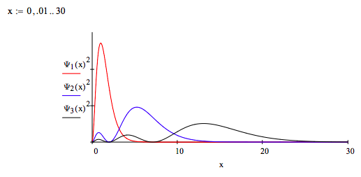
The following exercises pertain to several of the 1 = 0 states of the one-dimensional hydrogen atom.

\[ \begin{matrix} 1s & \Psi_1 (x) = 2 x \text{exp}(-x) & 2s & \Psi_2 (x) = \frac{1}{ \sqrt{8}} x (2-x) \text{exp} \left( - \frac{x}{2} \right) \\ 3s & \Psi_3 (x) = \frac{2}{243} \sqrt{3} x \left( 27-18x + 2x^2 \right) \text{exp} \left( - \frac{x}{3} \right) \end{matrix} \nonumber \]

Coordinate Space Calculations

\[ \begin{matrix} \text{Position operator:} & x \blacksquare & \text{Momentum operator:} & p = \frac{1}{i} \frac{d}{dx} \blacksquare & \text{Integral:} & \int_0 ^{ \infty} \blacksquare dx \\ \text{Kinetic energy operator:} & KE = - \frac{1}{2} \frac{d^2}{dx^2} & \text{Potential energy operator:} & PE = \frac{-1}{x} \blacksquare \end{matrix} \nonumber \]

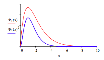
Plot Ψ(x) and Ψ(x)²:

Show that this wave function is normalized:

\[ \begin{matrix} \int_0^{ \infty} \Psi_1 (x)^2 dx \rightarrow 1 & \int_0^{ \infty} \Psi_1 (x)^2 dx = 1 \end{matrix} \nonumber \]

Calculate the most probable position for the electron:

\[ \frac{d}{dx} (2 \text{x exp(-x))} = 0 \text{solve, x} \rightarrow 1 \nonumber \]

Calculate the average value of the electron position:

\[ \int_0^{ \infty} \Psi_1 (x) x \Psi_1 (x) dx \rightarrow \frac{3}{2} \nonumber \]

Calculate the probability density at both the most probable and average positions of the electron:

\[ \begin{matrix} \text{Most probable:} & \Psi_1 (x)^2 = 0.541 & \text{Average:} & \Psi_1 \left( \frac{3}{2} \right)^2 = 0.448 \end{matrix} \nonumber \]

Calculate the probability that the electron is between the nucleus and the most probable value of the electron position:

\[ \begin{matrix} \int_0^1 \Psi_1 (x)^2 \text{dx float, 3} \rightarrow 0.323 & \int_0^1 \Psi_1 (x)^2 dx = 0.323 \end{matrix} \nonumber \]

Calculate the probability that the electron is between the nucleus and the average value of the electron position:

\[ \begin{matrix} \int_0^{ \frac{3}{2}} \Psi_1 (x)^2 \text{dx float, 3} \rightarrow 0.577 & \int_0^{ \frac{3}{2}} \Psi_1 (x)^2 dx = 0.577 \end{matrix} \nonumber \]

Calculate the probability that the electron is beyond the most probable position:

\[ \begin{matrix} \int_1^{ \infty} \Psi_1 (x)^2 \text{dx float, 3} \rightarrow 0.677 & \int_1 ^{ \infty} \Psi_1 (x)^2 dx = 0.677 \end{matrix} \nonumber \]

Calculate the probability that the electron will be found inside the nucleus. The nuclear dimension is approximately 2 x 10^-5 a_o.

\[ \int_0^{.00002} \Psi_1 (x)^2 dx = 1.067 \times 10^{-14} \nonumber \]

Calculate that position from the nucleus for which the probability of finding the electron is 0.95:

\[ \begin{matrix} a = 2 & \text{Given} & \int_0^a \Psi_1 (x)^2 dx = .95 & \text{Find(a)} = 3.148 \end{matrix} \nonumber \]

Calculate the uncertainty in position:

\[ \Delta x = \sqrt{ \int_0^{ \infty} \Psi_1 (x)x^2 \Psi_1 (x) dx - \left( \int_0^{ \infty} \Psi_1 (x) x \Psi_1 (x) dx \right)^2} \text{float, 3} \rightarrow 0.866 \nonumber \]

Calculate the average value of the electronic momentum:

\[ \int_0 ^{ \infty} \Psi_1 (x) \frac{1}{i} \frac{d}{dx} \Psi_1 (x) dx \rightarrow 0 \nonumber \]

Calculate the uncertainty in momentum:

\[ \Delta p = \sqrt{ \int_0^{ \infty} \Psi_1 (x) - \frac{d^2}{dx^2} \Psi_1 (x) dx - \left( \int_0^{ \infty} \Psi_1 (x) \frac{1}{i} \frac{d}{dx} \Psi_1 (x) dx \right)^2} \rightarrow 1 \nonumber \]

Demonstrate that the position-momentum uncertainty relation is obeyed:

\[ \Delta x \Delta p = 0.866 \nonumber \]

This value is greater than .5 as required.

Calculate the position-momentum commutator. Interpret the result.

\[ \frac{x \left( \frac{1}{i} \frac{d}{dx} \Psi_1 (x) \right) - \frac{1}{i} \frac{d}{dx} \left( x \Psi_1 (x) \right)}{ \Psi_1 (x)} \text{simplify} \rightarrow i \nonumber \]

Position and momentum measurements do not commute. The wave function is not an eigenfunction of the position and momentum operators.

Calculate the average value for kinetic energy:

\[ \begin{matrix} \int_0 ^{ \infty} \Psi_1 (x) - \frac{1}{2} \frac{d^2}{dx^2} \Psi_1 (x) dx \rightarrow \frac{1}{2} & \int_0 ^{ \infty} \Psi_1 (x) - \frac{1}{2} \frac{d^2}{dx^2} \Psi_1 (x) dx = 0.5 \end{matrix} \nonumber \]

Calculate the average value for potential energy:

\[ \begin{matrix} \int_0 ^{ \infty} \Psi_1 (x) - \frac{1}{x} \frac{d^2}{dx^2} \Psi_1 (x) dx \rightarrow -1 & \int_0 ^{ \infty} \Psi_1 (x) - \frac{1}{x} \frac{d^2}{dx^2} \Psi_1 (x) dx = -1 \end{matrix} \nonumber \]

Calculate the average value for the total energy: \( \frac{1}{2} - 1 = -0.5 \) or

\[ \begin{matrix} \int_0 ^{ \infty} \Psi_1 (x) - \frac{1}{2} \frac{d^2}{dx^2} \Psi_1 (x) dx \rightarrow \frac{1}{2} & \int_0 ^{ \infty} \Psi_1 (x) - \frac{1}{x} dx \Psi_1 (x) dx = - \frac{1}{2} \end{matrix} \nonumber \]

These results illustrate the virial theorem:

\[ E = -T = \frac{V}{2} \nonumber \]

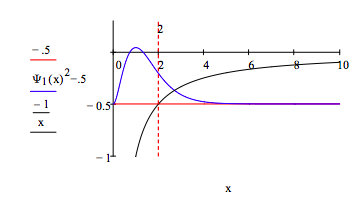
Calculate the probability that the electron is in a classically forbidden region, that is a region for which E < V. First show that the classically forbidden region begins at x = 2, where E = V. For x larger than 2 the potential energy will be greater than the total energy. This is an example of quantum mechanical tunneling. Show the classically forbidden region graphically.

\[ \begin{matrix} \frac{-1}{2} = \frac{-1}{x} \text{ solve, x } \rightarrow 2 & \int_2^{ \infty} \Psi_1 (x)^2 dx = 0.238 \end{matrix} \nonumber \]

Demonstrate that the wave function is not an eigenfunction of the kinetic energy operator and comment on the significance of this result:

\[ \frac{- \frac{1}{2} \frac{d^2}{dx^2} \Psi_1 (x) - \frac{1}{x} \Psi_1 (x)}{ \Psi_1 (x)} \text{simplify} \rightarrow \frac{1}{x} - \frac{1}{2} \nonumber \]

Electron in the hydrogen atom does not have a well-defined value for kinetic energy.

Demonstrate that the wave function is not an eigenfunction of the potential energy operator and comment on the significance of this result:

\[ \frac{- \frac{1}{2} \frac{d^2}{dx^2} \Psi_1 (x) - \frac{1}{x} \Psi_1 (x)}{ \Psi_1 (x)} \text{simplify } \rightarrow - \frac{1}{2} \nonumber \]

In spite of not having a well-defined kinetic or potential energy, the electron in the hydrogen atom has a well-defined total energy.

\[ - \frac{1}{2} \frac{d}{dx^2} \Psi_1 (x) - \frac{1}{x} \Psi_1 (x) = E \Psi_1 (x) \text{ solve, E} \rightarrow - \frac{1}{2} \nonumber \]

What is the energy eigenvalue and how does it compare to previous calculations in this exercise:

The energy eigenvalue is -0.5 which is in agreement with + calculated previously.

Calculate the overlap integral with the 2s orbital:

\[ \int_0^{ \infty} \Psi_1 (x) \Psi_2 (x) dx \rightarrow 0 \nonumber \]

Interpret the result: the orbitals are orthogonal.

Calculate the kinetic, potential and total energy of a 2s electron and show that the virial theorem is satisfied.

\[ \begin{matrix} \int_0^{ \infty} \Psi_2 (x) - \frac{1}{2} \frac{d^2}{dx^2} \Psi_2 (x) dx \rightarrow \frac{1}{8} & \int_0^{ \infty} \Psi_2 (x) - \frac{1}{x} \Psi_2 (x) dx \rightarrow - \frac{1}{4} & F = \frac{1}{8} - \frac{1}{4} & F \rightarrow - \frac{1}{8} \end{matrix} \nonumber \]

\[ E = -T =\frac{V}{2} \nonumber \]

Calculate the kinetic, potential and total energy of a 3s electron and show that the virial theorem is satisfied.

\[ \begin{matrix} \int_0^{ \infty} \Psi_3 (x) - \frac{1}{2} \frac{d^2}{dx^2} \Psi_3 (x) dx \rightarrow \frac{1}{18} & \int_0^{ \infty} \Psi_3 (x) - \frac{1}{x} \Psi_3 (x) dx \rightarrow - \frac{1}{9} & E = \frac{1}{18} - \frac{1}{9} & E \rightarrow - \frac{1}{18} \end{matrix} \nonumber \]

\[ E = -T =\frac{V}{2} \nonumber \]

Plot the 1s and 2s orbitals on the same graph and explain the orthogonality or net zero overlap.

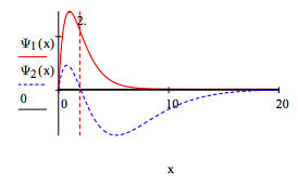
From x = 0 to 2 the overlap is positive, and x=2 to ∞ it is equal in magnitude but negative.

\[ \begin{matrix} \int_0^2 \Psi_1 (x) \Psi_2 (x) dx = 0.188 \\ \Psi_2^{ \infty} \Psi_1 (x) \Psi_2 (x) dx = -0.188 \end{matrix} \nonumber \]

Momentum Space Calculations

Fourier transform the 1s coordinate-space wave function into momentum space.

\[ \Phi_1 (p) = \frac{1}{ \sqrt{2 \pi}} \left( \int_0^{ \infty} \text{exp} (-ipx) \Psi_1 (x) dx \right) \rightarrow \frac{ \sqrt{2}}{ \sqrt{ \pi} (1 + pi)^2} \nonumber \]

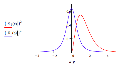
Plot |Ψ(x)|² and |Φ(p)|² on the same graph:

\[ \begin{matrix} p = -5,~-4.99, ... 5 & x = 0,~.01 .. 5 \end{matrix} \nonumber \]

\[ \begin{matrix} \text{Momentum space integral:} & \int_{ - \infty}^{ \infty} \blacksquare dp & \text{Momentum operator:} & p \blacksquare \\ \text{Kinetic energy operator:} & \frac{p^2}{2} & \text{Position operator:} & i \frac{d}{dp} \blacksquare \end{matrix} \nonumber \]

Demonstrate that the 1s momentum wavefunction is normalized.

\[ \begin{matrix} \int_{- \infty}^{ \infty} \overline{ \Phi_1 (p)} \Psi_1 (p) dp = 1 & \text{or} & \int_{ - \infty}^{ \infty} \left( \left| \Psi_1 (p) \right| \right)^2 = 1 \end{matrix} \nonumber \]

Calculate the average value of the momentum and compare it to value obtained with the coordinate space wave function.

\[ \begin{matrix} \int_{- \infty}^{ \infty} \overline{ \Phi_1 (p)} \Psi_1 (p) dp = 1 & \text{Same value} \end{matrix} \nonumber \]

Calculate the average value of the kinetic energy and compare it to value obtained with the 1s coordinate space wave function.

\[ \begin{matrix} \int_{- \infty}^{ \infty} \overline{ \Phi_1 (p)} \frac{p^2}{2} \Psi_1 (p) dp = 0.5 & \text{Same value} \end{matrix} \nonumber \]

Calculate the average value of the electron position and compare it to value obtained with the 1s coordinate space wave function.

\[ \begin{matrix} \int_{- \infty}^{ \infty} \overline{ \Phi_1 (p)} i \frac{p}{dp} \Psi_1 (p) dp = 1.5 & \text{Same value} \end{matrix} \nonumber \]

Calculate the uncertainty in position using the momentum wave function:

\[ \begin{matrix} \int_{- \infty}^{ \infty} \overline{ \Phi_1 (p)} - \frac{d^2}{dp^2} \Phi_1 (p) dp = 3 & \Delta x = \sqrt{3 - \left( \frac{3}{2} \right)^2} & \Delta x = 0.866 \end{matrix} \nonumber \]

Calculate the uncertainty in momentum using the momentum wave function:

\[ \begin{matrix} \int_{- \infty}^{ \infty} \overline{ \Phi_1 (p)} - \frac{d^2}{dp^2} \Phi_1 (p) dp = 3 & \Delta p = \sqrt{1-0} & \Delta p = 1 \end{matrix} \nonumber \]

Demonstrate that the position-momentum uncertainty relation is satisfied:

\[ \begin{matrix} \Delta x \Delta p = 0.866 & \text{Same value.} \end{matrix} \nonumber \]

Fourier transform the 2s wavefunction into momentum space:

\[ \Phi_2 (p) = \frac{1}{ \sqrt{2 \pi}} \int_0^{ \infty} \text{exp} (-ipx) \Psi_2 (x) \text{dx simplify} \rightarrow \frac{2(-1 + 2ip)}{ \sqrt{ \pi} (1+2ip)^3} \nonumber \]

Demonstrate the 2s wavefunction is normalized.

\[ \int_{ - \infty}^{ \infty} \left( \left| \Phi_2 (p) \right| \right)^2 dp = 1 \nonumber \]

Demonstrate the 1s and 2s momentum wavefunctions are orthogonal.

\[ \int_{ \infty}^{ \infty} \overline{ \Phi_1 (p)} \Phi_2 (p) dp = 0 \nonumber \]

Fourier transform the 3s wavefunction into momentum space.

\[ \Phi_3 (p) = \frac{1}{ \sqrt{2 \pi}} \int_0 ^{ \infty} \text{exp}(-ipx) \Psi_3 (x) \text{dx simplify } \rightarrow \frac{ \sqrt{6} (-1 + 3ip)^2}{ \sqrt{ \pi} (1 +3ip)^4} \nonumber \]

Demonstrate the 3s momentum wavefunction is normalized.

\[ \int_{ - \infty}^{ \infty} \left( \left| \Phi_3 (p) \right| \right)^2 dp = 1 \nonumber \]

Plot the 1s, 2s and 3s momentum wavefunctions and interpret the graph in terms of the uncertainty principle.

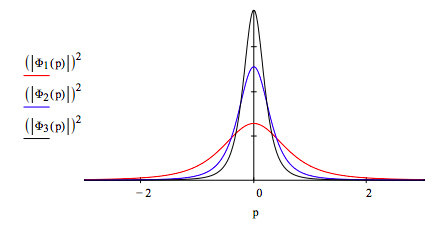
As shown below, as the principal quantum number increases, the spatial distribution of the electron becomes more delocalized. Therefore, according to the uncertainty principle, the momentum distribution must become more localized. The graph above shows a more localized momentum distribution as the principle quantum number increases.