2.3: The de Broglie-Bohr Model for the Hydrogen Atom - Version 3
- Page ID
- 154848
The 1913 Bohr model of the hydrogen atom was replaced by Schrödinger's wave mechanical model in 1926. However, Bohr's model is still profitably taught today because of its conceptual and mathematical simplicity, and because it introduced a number of key quantum mechanical ideas such as the quantum number, quantization of observable properties, quantum jump and stationary state.
Bohr calculated the manifold of allowed electron energies by balancing the mechanical forces (centripetal and electron-nucleus) on an electron executing a circular orbit of radius R about the nucleus, and then arbitarily quantizing its angular momentum. Finally by fiat he declared that the electron was in a non-radiating stationary state because an orbiting (accelerating) charge radiates energy and will collapse into the oppositely charge nucleus.
In 1924 de Broglie postulated wave-particle duality for the electron and thereby provided the opportunity to take some of the arbitariness out of Bohr's model. An electron possessing wave properties is subject to constructive and destructive interference. As will be shown this leads naturally to quantization of electron momentum and kinetic energy, and consequently a manifold of allowed energy states for the electron relative to the nucleus.
The de Broglie-Bohr model of the hydrogen atom presented here treats the electron as a particle on a ring with wave-like properties. The electron's kinetic (confinement) energy is calculated using its momentum eigenfunction in the coordinate representation. This equation is obtained by substituting the de Broglie wave-particle equation (λ = h/p) into Euler's equation, the most general one-dimensional wavefunction.
\[ \begin{matrix} \langle x | \lambda \rangle = \frac{1}{ \sqrt{2 \pi}} \text{exp} \left( \frac{i2 \pi x}{ \lambda} \right) & \text{plus} & \lambda = \frac{h}{p} & \text{yields} & \langle x | p \rangle = \frac{1}{ \sqrt{2 \pi}} \text{exp} \end{matrix} \nonumber \]
In order to avoid destructive interference, the electron's momentum wavefunction must be single-valued, which in this application requires a circular boundary condition: the wavefunction must match at points separated by one circumference, 2 πr. The mathematical consequence of satisfying this requirement leads to quantized momentum and the emergence of a quantum number, n.
\[ \begin{matrix} & \langle x + 2 \pi r | p \rangle = \langle x | p \rangle & \\ \text{exp} \left( \frac{ip(x+2 \pi r)}{ \hbar} \right) = \text{exp} \left( \frac{ipx}{ \hbar} \right) & & \text{exp} \left( \frac{ipx}{ \hbar} \right) \text{exp} \left( \frac{i2 \pi p r}{ \hbar} \right) = \text{exp} \left( \frac{ipx}{ \hbar} \right) \\ & \text{exp} \left( \frac{i2 \pi p r}{ \hbar} \right) = 1 \end{matrix} \nonumber \]
The last equation succinctly states the boundary condition requirements and is satisfied when,
\[ \begin{matrix} \frac{pr}{ \hbar} = \frac{mvr}{ \hbar} = n & \text{where} & n = 0,~ \pm 1,~ \pm 2 ... \end{matrix} \nonumber \]
This restriction quantizes the angular momentum and allows the conversion of classical kinetic energy into its quantum mechanical form. In this model, the +/- values suggest clockwise and counter-clockwise angular momentum.
\[ \begin{matrix} T_n = \frac{p^2}{2m} = \frac{n^2 \hbar^2}{2m r^2} & \text{where} & n = 0,~ \pm 1,~ \pm 2 ... \end{matrix} \nonumber \]
The wavefunctions associated with these quantized kinetic energies are obtained by using the quantum condition of equation 3 to eliminate momentum in equation 1, recognizing that in radians θ = x/R. (x is the linear distance on the ring from some reference point.)
\[ \Psi_n ( \theta ) = \langle \theta | n \rangle = \frac{1}{ \sqrt{2 \pi}} \text{exp} ( in \theta ) \nonumber \]
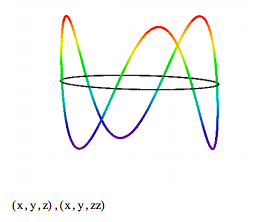
The allowed electron wavefunctions are displayed graphically as follows.
\[ \begin{matrix} \text{Quantum number:} & n = 3 \\ \text{numpts = 200} & i = 0 ... \text{numpts} & j = 0 ... \text{numpts} & \theta_i = \frac{2 \pi i}{ \text{numpts}} \end{matrix} \nonumber \]

The quantum mechanical interpretation of these "Bohr orbits" is that they are stationary states. In spite of the fact that we use the expression kinetic energy, which implies electron motion, there is no motion. The electron occupies the orbit as a particle-wave, it is not orbiting the nucleus. If it was orbiting in a classical sense it would radiate energy and quickly collapse into the nucleus. Clearly the stability of matter requires the quantum mechanical version of kinetic energy.
We now place a proton at the center of the ring and calculate the potential energy using Coulombs law.
\[ V = - \frac{e^2}{4 \pi \varepsilon_0 r} \nonumber \]
Adding the kinetic and potential energy terms yields the total energy. However, the n = 0 state is discarded because it has zero kinetic energy and therefore does not represent a stable atomic state.
\[ E = T + V = \frac{n^2 h^2}{* \pi^2 m_e r^2} - \frac{e^2}{4 \pi \varepsilon_0 r} \nonumber \]
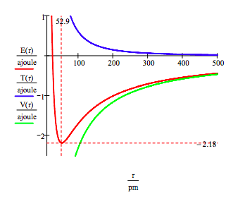
The ground state energy and orbit radius of the electron in the hydrogen atom is found by plotting the energy as a function of the orbital radius. The ground state is the minimum in the total energy curve. Naturally calculus can be used to obtain the same information by minimizing the energy with respect to the orbit radius. However, the graphical method has the virtue of illuminating the issue of atomic stability.
Fundamental constants: electron charge, electron mass, Planck's constant, vacuum permitivity.
\[ \begin{matrix} e = 1.6021777 (10)^{-19} \text{coul} & m_e = 9.10939 (10)^{-31} \text{kg} \\ h = 6.62608 (10)^{-34} \text{joule sec} & \varepsilon_0 = 8.85419 (10)^{-12} \frac{ \text{coul}^2}{ \text{joule m}} \end{matrix} \nonumber \]
Quantum number and conversion factor between meters and picometers and joules and attojoules.
\[ \begin{matrix} n = 1 & pm = (10)^{-12} m & \text{ajoule} = 10^{-18} \text{joule} \end{matrix} \nonumber \]
\[ \begin{matrix} r = 20 pm,~20.5 pm .. 500 pm & T(r) = \frac{n^2 h^2}{8 \pi^2 m_e r^2} & V(r) = - \frac{e^2}{4 \pi \varepsilon_0 r} & E(r) = T(r) + V(r) \end{matrix} \nonumber \]

This figure shows that atomic stability involves a balance between potential and kinetic energy. The electron is drawn toward the nucleus by the attractive potential energy interaction (~ -1/R), but is prevented from collapsing into the nucleus by the extremely large kinetic energy (~1/R 2) associated with small orbits.
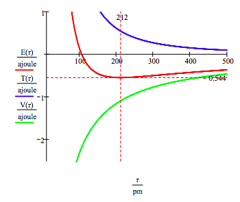
As shown below, the graphical approach can also be used to find the electronic excited states.
\[ \begin{matrix} n = 2 & T(r) = \frac{n^2 h^2}{8 \pi^2 m_e r^2} & V(r) = - \frac{e^2}{4 \pi \varepsilon_0 r} & E(r) = T(r) + V(r) \end{matrix} \nonumber \]

However, it is much easier to generate the manifold of allowed electron energies by minimizing the energy with respect to the orbit radius. This procedure yields,
\[ \begin{matrix} E_n = - \frac{m_e e^4}{2 \left( 4 \pi \varepsilon_0 \right)^2 \hbar^2} \frac{1}{n} & \text{and} & r_n = \frac{4 \pi \varepsilon_0 \hbar^2}{m_e e^2} n^2 \end{matrix} \nonumber \]

