1.83: Demonstrating the Uncertainty Priniciple for Angular Momentum and Angular Position
- Page ID
- 157391
The uncertainty relation between angular momentum and angular position can be derived from the more familiar uncertainty relation between linear momentum and position.
\[
\Delta \mathrm{p} \cdot \Delta \mathrm{x} \geq \frac{\mathrm{h}}{4 \cdot \pi} \tag{1}
\nonumber \]
Consider a particle with linear momentum p moving on a circle of radius r. The particleʹs angular momentum is given by equation (2).
\[
\mathrm{L}=\mathrm{m} \cdot \mathrm{v} \cdot \mathrm{r}=\mathrm{p} \cdot \mathrm{r} \tag{2}
\nonumber \]
In moving a distance x on the circle the particle sweeps out an angle \(\phi\) in radians.
\[
\phi=\frac{x}{r} \tag{3}
\nonumber \]
Equations (2) and (3) suggest,
\[
\Delta \mathrm{p}=\frac{\Delta \mathrm{L}}{\mathrm{r}} \qquad \Delta \mathrm{x}=\Delta \phi \cdot \mathrm{r} \tag{4}
\nonumber \]
Substitution of equations (4) into equation (1) yields the angular momentum, angular position uncertainty relation.
\[
\Delta \mathrm{L} \cdot \Delta \phi \geq \frac{\mathrm{h}}{4 \cdot \pi} \tag{5}
\nonumber \]
In addition to the Heisenberg restrictions represented by equations (1) and (5), conjugate observables are related by Fourier transforms. For example, for position and momentum it is given by equation (6) in atomic units (h = 2\(\pi\)).
\[
\langle p | x\rangle=\frac{1}{\sqrt{2 \pi}} \exp (-i p x) \tag{6}
\nonumber \]
Equations (2) and (3) can be used with (6) to obtain the Fourier transform between angular momentum and angular position.
\[
\langle L | \phi\rangle=\frac{1}{\sqrt{2 \pi}} \exp (-i L \phi) \tag{7}
\nonumber \]
Equations (6) and (7) are mathematical dictionaries telling us how to translate from x language to p language, or \(\phi\) language to L language. The complex conjugates of (6) and (7) translate in the reverse direction, from p to x and from L to \(\phi\).
The work‐horse particle‐in‐a‐box (PIB) problem can be used to provide a compelling graphical illustration of the position‐momentum uncertainty relation. The position wave function for the ground state of a PIB in a box of length a is given below.
\[
\langle x | \Psi\rangle=\sqrt{\frac{2}{a}} \sin \left(\frac{\pi x}{a}\right) \tag{8}
\nonumber \]
The conjugate momentum‐space wave function is obtained by the following Fourier transform.
\[
\langle p | \Psi\rangle=\int_{0}^{a}\langle p | x\rangle\langle x | \Psi\rangle d x=\frac{1}{\sqrt{\pi a}} \int_{0}^{a} \exp (-i p x) \sin \left(\frac{\pi x}{a}\right) \tag{9}
\nonumber \]
Evaluation of the integral in equation (9) yields,
\[
\Psi(p, a) :=\sqrt{a \cdot \pi} \cdot \frac{\exp (-i \cdot p \cdot a)+1}{\pi^{2}-p^{2} \cdot a^{2}} \tag{10}
\nonumber \]
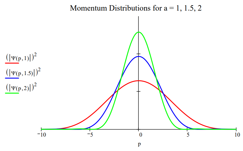
Plotting the momentum distribution function for several box lengths, as is done in the figure below, clearly reveals the position‐momentum uncertainty relation. The greater the box length the greater the uncertainty in position. However, as the figure shows, the greater the box length the narrower the momentum distribution, and, consequently, the smaller the uncertainty in momentum.
A similar visualization of the angular‐momentum/angular‐position uncertainty relation is also possible. Suppose a particle on a ring is prepared in such a way that its angular wave function is represented by the following gaussian function,
\[
\langle\phi | \Psi\rangle=\exp \left(-a \phi^{2}\right) \tag{11}
\nonumber \]
where the parameter a controls the width of the angular distribution. The conjugate angular momentum wave function is obtained by the following Fourier transform.
\[
\langle L | \Psi\rangle=\int_{-\pi}^{\pi}\langle L | \phi\rangle\langle\phi | \Psi\rangle d \phi=\frac{1}{\sqrt{2 \pi}} \int_{-\pi}^{\pi} \exp (-i L \phi) \exp \left(-a \phi^{2}\right) d \phi \tag{12}
\nonumber \]
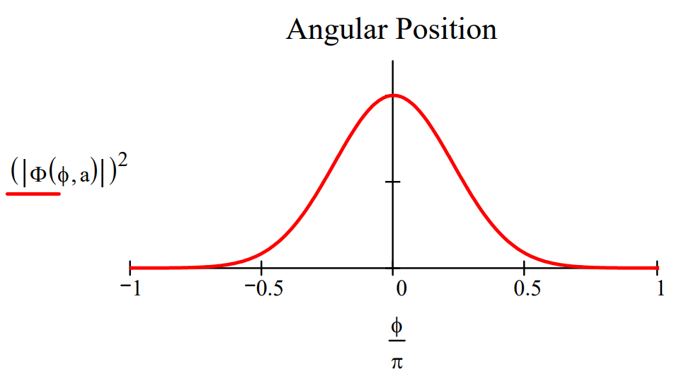
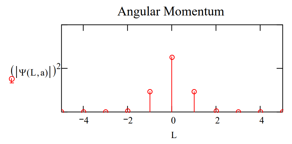
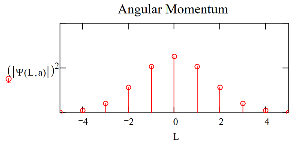
Plots of \(|<\phi| \Psi>\left.\right|^{2}\) and \(|<\mathrm{L}| \Psi>\left.\right|^{2}\) shown below for two values of the parameter a illustrate the angular momentum/angular position uncertainty relation. The larger the value of a, the smaller the angular positional uncertainty and the greater the angular momentum uncertainty. In other words, the greater the value of a the greater the number of angular momentum eigenstates observed.
\[
\mathrm{a} :=0.5 \qquad \Phi(\phi, \mathrm{a}) :=\exp \left(-\mathrm{a} \cdot \phi^{2}\right)
\nonumber \]
\[
\mathrm{L} :=-5 \ldots 5 \qquad \Psi(\mathrm{L}, \mathrm{a}) :=\int_{-\pi}^{\pi} \exp (-\mathrm{i} \cdot \mathrm{L} \cdot \phi) \Phi(\phi, \mathrm{a}) \mathrm{d} \phi
\nonumber \]
Make the angular position distribution narrower: \(a :=2.5\)
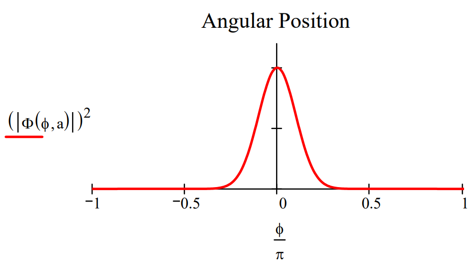
Observe a broader distribution in angular momentum.
The uncertainty relation between angular position and angular momentum as outlined above is a simplified version of that presented by S. Franke‐Arnold et al. in New Journal of Physics 6, 103 (2004).

