1.80: Another view of the Harmonic Oscillator and the Uncertainty Principle

Schrödinger's equation in atomic units (h = 2\(\pi\)) for the harmonic oscillator has an exact analytical solution.

\[
\mathrm{V}(\mathrm{x}, \mathrm{k}) :=\frac{1}{2} \cdot \mathrm{k} \cdot \mathrm{x}^{2} \qquad \frac{-1}{2 \cdot \mu} \cdot \frac{\mathrm{d}^{2}}{\mathrm{dx}^{2}} \Psi(\mathrm{x})+\mathrm{V}(\mathrm{x}) \cdot \Psi(\mathrm{x})=\mathrm{E} \cdot \Psi(\mathrm{x})
\nonumber \]

The ground-state wave function (coordinate space) and energy for an oscillator with reduced mass \(\mu\) and force constant k are as follows.

\[
\Psi(x, k, \mu) :=\left(\frac{\sqrt{k \cdot \mu}}{\pi}\right)^{\frac{1}{4}} \cdot \exp \left(-\sqrt{k \cdot \mu} \cdot \frac{x^{2}}{2}\right) \qquad E(k, \mu) :=\frac{1}{2} \cdot \sqrt{\frac{k}{\mu}}
\nonumber \]

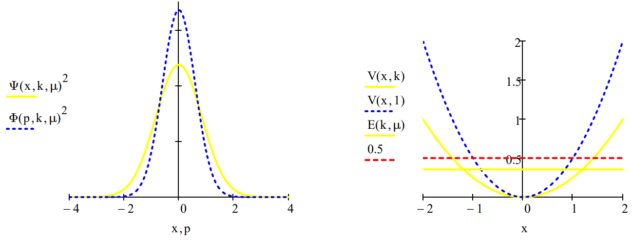
The first thing we want to illustrate is that tunneling occurs in the simple harmonic oscillator. The classical turning point is that position at which the total energy is equal to the potential energy. In other words, classically the kinetic energy is zero and the oscillator's direction is going to reverse. For the ground state the classical turning point is,

\[
\frac{1}{2} \cdot \sqrt{\frac{\mathrm{k}}{\mu}}=\frac{1}{2} \cdot \mathrm{k} \cdot \mathrm{x}^{2} \quad \text{has solution(s)} \begin{pmatrix} \frac{-1}{k^{\frac{1}{4}} \cdot \mu^{\frac{1}{4}}} \\ \frac{1}{k^{\frac{1}{4}} \cdot \mu^{\frac{1}{4}}}\end{pmatrix}
\nonumber \]

From the quantum mechanical perspective the oscillator is not vibrating; it is in a stationary state. To the extent that the oscillator's wave function extends beyond the classical turning point, tunneling is occurring. The calculation below shows that the probability that tunneling occurs is independent of the values of k and \(\mu\) for the ground state.

\[
2 \cdot \left[ \int_{\frac{1}{(k \cdot \mu)^{\frac{1}{4}}}}^{\infty} \left[ \left(\frac{\sqrt{k\cdot\mu}}{\pi}\right)^{\frac{1}{4}}\cdot\exp\left(- \sqrt{k\cdot\mu}\cdot\frac{x^{2}}{2}\right)\right]^{2}dx\right] \Bigg|_{\text{simplify}}^{\text{assume,} k>0, \; \mu > 0} \rightarrow 1 - \text{erf} (1)=0.157
\nonumber \]

A Fourier transform of the coordinate wave function provides its counter part in momentum space.

\[
\Phi(\mathrm{p}, \mathrm{k}, \mu) :=\frac{1}{\sqrt{2 \cdot \pi}} \cdot \int_{-\infty}^{\infty} \exp (-\mathrm{i} \cdot \mathrm{p} \cdot \mathrm{x}) \cdot \Psi(\mathrm{x}, \mathrm{k}, \mu) \mathrm{d} \mathrm{x} \Bigg| \begin{array}{l}{\text { assume, } \mathrm{k}>0} \\ {\text { assume, } \mu>0} \\ {\text { simplify }}\end{array}\rightarrow\frac{e^{-\frac{p^{2}}{2 \cdot \sqrt{\mu} \cdot \sqrt{k}}}}{\pi^{\frac{1}{4}} \cdot \mu^{\frac{1}{8}} \cdot k^{\frac{1}{8}}}
\nonumber \]

The uncertainty principle can now be illustrated by comparing the coordinate and momentum wave functions for a variety values of k and \(\mu\). For the benchmark case, k = \(\mu\) = 1, we see that the coordinate and momentum wave functions are identical and the classical turning point (CTP) is 1. The classical turning point will be taken as a measure of the spatial domain of the oscillator.

• For k = 2 and \(\mu\) =1, the force constant has doubled reducing the amplitude of vibration (CTP =0.841) and therefore the uncertainty in position. Consequently there is an increase in the uncertainty in momentum which is manifested by a broader momentum distribution function.
• For k = 1 and \(\mu\) = 2, the increase in effective mass drops the oscillator in the potential well decreasing the vibrational amplitude (CTP = 0.841) causing a decrease in \(\Delta\)x and an increase in \(\Delta\)p.
• For k = 0.5 and \(\mu\) = 1, the lower force constant causes a larger vibrational amplitude (CTP = 1.189) and an accompanying increase in \(\Delta\)x. Consequently \(\Delta\)p decreases.

Force constant: \(k : = 0.5\)	Effective mass: \(\mu : = 1\)
Energy: \(\mathrm{E}(\mathrm{k}, \mu)=0.354\)	CTP: \(\frac{1}{k^{\frac{1}{4}} \cdot \mu^{\frac{1}{4}}}=1.189\)

The uncertainties in position and momentum are calculated as shown below because for the harmonic oscillator <x> =

= 0.

\[
\Delta x :=\sqrt{\int_{-\infty}^{\infty} x^{2} \cdot \Psi(x, k, \mu)^{2} d x}=0.841 \\ \Delta p :=\sqrt{\int_{-\infty}^{\infty} p^{2} \cdot \Phi(p, k, \mu)^{2} d p}=0.595 \\ \Delta x \cdot \Delta p=0.5
\nonumber \]

A summary of the four cases considered is provided in the table below.

\[
\left(\begin{array}{cccccc}{\mu} & {k} & {C T P} & {\Delta x} & {\Delta p} & {\Delta x \Delta p} \\ {1} & {1} & {1.00} & {0.707} & {0.707} & {0.5} \\ {1} & {2} & {0.841} & {0.595} & {0.841} & {0.5} \\ {2} & {1} & {0.841} & {0.595} & {0.841} & {0.5} \\ {1} & {0.5} & {1.189} & {0.841} & {0.594} & {0.5}\end{array}\right)
\nonumber \]

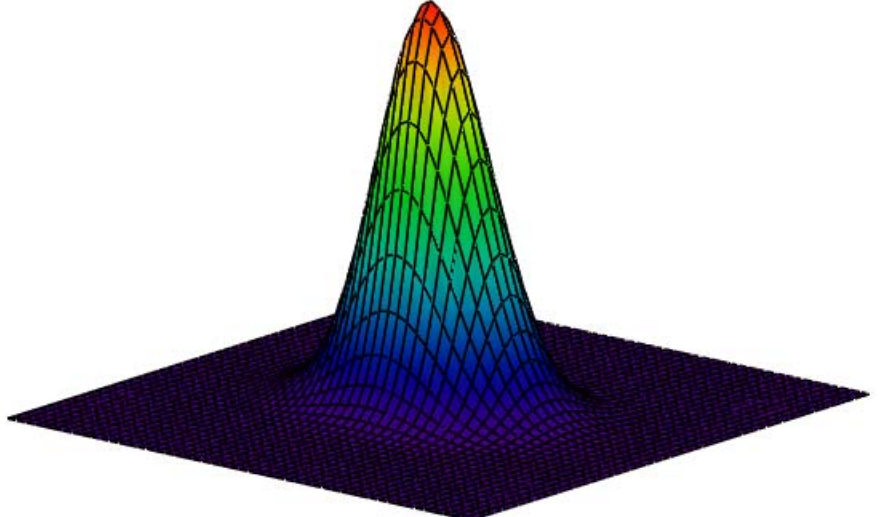
The Wigner function, W(x,p), is a phase-space distribution that can be used to provide an alternative graphical representation of the results calculated above. As shown below it can be generated using either the coordinate or momentum wave function.

Calculate Wigner distribution:

\[
\mathrm{W}(\mathrm{x}, \mathrm{p}) :=\frac{1}{\pi^{\frac{3}{2}}} \cdot \int_{-\infty}^{\infty} \Psi\left(\mathrm{x}+\frac{\mathrm{s}}{2}, \mathrm{k}, \mu\right) \cdot \exp (\mathrm{i} \cdot \mathrm{s} \cdot \mathrm{p}) \cdot \Psi\left(\mathrm{x}-\frac{\mathrm{s}}{2}, \mathrm{k}, \mu\right) \mathrm{ds}
\nonumber \]

Display Wigner distribution:

\[
\mathrm{N} :=50 \qquad \mathrm{i} :=0 \ldots \mathrm{N} \qquad \mathrm{x}_{\mathrm{i}} :=-4+\frac{8 \cdot \mathrm{i}}{\mathrm{N}} \\ \mathrm{j} :=0 \ldots \mathrm{N} \qquad \mathrm{p}_{\mathrm{j}} :=-4+\frac{8 \cdot \mathrm{j}}{\mathrm{N}} \qquad \text{Wigner}_{\mathrm{i},\mathrm{j}} :=\mathrm{W}\left(\mathrm{x}_{\mathrm{i}}, \mathrm{p}_{\mathrm{j}}\right)
\nonumber \]

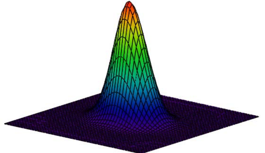
Calculate Wigner distribution:

\[
\mathrm{W}(\mathrm{x}, \mathrm{p}) :=\frac{1}{\pi^{\frac{3}{2}}} \cdot \int_{-\infty}^{\infty} \Phi\left(\mathrm{p}+\frac{\mathrm{s}}{2}, \mathrm{k}, \mu\right) \cdot \exp (\mathrm{i} \cdot \mathrm{s} \cdot \mathrm{x}) \cdot \Phi\left(\mathrm{p}-\frac{\mathrm{s}}{2}, \mathrm{k}, \mu\right) \mathrm{ds}
\nonumber \]

Display Wigner distribution:

\[
\mathrm{N} :=50 \qquad \mathrm{i} :=0 \ldots \mathrm{N} \qquad \mathrm{x}_{\mathrm{i}} :=-4+\frac{8 \cdot \mathrm{i}}{\mathrm{N}} \\ \mathrm{j} :=0 \ldots \mathrm{N} \quad \mathrm{p}_{\mathrm{j}} :=-4+\frac{8 \cdot \mathrm{j}}{\mathrm{N}} \qquad \text{Wigner}_{\mathrm{i}, \mathrm{j}} :=\mathrm{W}\left(\mathrm{x}_{\mathrm{i}}, \mathrm{p}_{\mathrm{j}}\right)
\nonumber \]