1.64: Wigner Distribution for the Double Slit Experiment
- Page ID
- 156418
\( \newcommand{\vecs}[1]{\overset { \scriptstyle \rightharpoonup} {\mathbf{#1}} } \)
\( \newcommand{\vecd}[1]{\overset{-\!-\!\rightharpoonup}{\vphantom{a}\smash {#1}}} \)
\( \newcommand{\id}{\mathrm{id}}\) \( \newcommand{\Span}{\mathrm{span}}\)
( \newcommand{\kernel}{\mathrm{null}\,}\) \( \newcommand{\range}{\mathrm{range}\,}\)
\( \newcommand{\RealPart}{\mathrm{Re}}\) \( \newcommand{\ImaginaryPart}{\mathrm{Im}}\)
\( \newcommand{\Argument}{\mathrm{Arg}}\) \( \newcommand{\norm}[1]{\| #1 \|}\)
\( \newcommand{\inner}[2]{\langle #1, #2 \rangle}\)
\( \newcommand{\Span}{\mathrm{span}}\)
\( \newcommand{\id}{\mathrm{id}}\)
\( \newcommand{\Span}{\mathrm{span}}\)
\( \newcommand{\kernel}{\mathrm{null}\,}\)
\( \newcommand{\range}{\mathrm{range}\,}\)
\( \newcommand{\RealPart}{\mathrm{Re}}\)
\( \newcommand{\ImaginaryPart}{\mathrm{Im}}\)
\( \newcommand{\Argument}{\mathrm{Arg}}\)
\( \newcommand{\norm}[1]{\| #1 \|}\)
\( \newcommand{\inner}[2]{\langle #1, #2 \rangle}\)
\( \newcommand{\Span}{\mathrm{span}}\) \( \newcommand{\AA}{\unicode[.8,0]{x212B}}\)
\( \newcommand{\vectorA}[1]{\vec{#1}} % arrow\)
\( \newcommand{\vectorAt}[1]{\vec{\text{#1}}} % arrow\)
\( \newcommand{\vectorB}[1]{\overset { \scriptstyle \rightharpoonup} {\mathbf{#1}} } \)
\( \newcommand{\vectorC}[1]{\textbf{#1}} \)
\( \newcommand{\vectorD}[1]{\overrightarrow{#1}} \)
\( \newcommand{\vectorDt}[1]{\overrightarrow{\text{#1}}} \)
\( \newcommand{\vectE}[1]{\overset{-\!-\!\rightharpoonup}{\vphantom{a}\smash{\mathbf {#1}}}} \)
\( \newcommand{\vecs}[1]{\overset { \scriptstyle \rightharpoonup} {\mathbf{#1}} } \)
\( \newcommand{\vecd}[1]{\overset{-\!-\!\rightharpoonup}{\vphantom{a}\smash {#1}}} \)
\(\newcommand{\avec}{\mathbf a}\) \(\newcommand{\bvec}{\mathbf b}\) \(\newcommand{\cvec}{\mathbf c}\) \(\newcommand{\dvec}{\mathbf d}\) \(\newcommand{\dtil}{\widetilde{\mathbf d}}\) \(\newcommand{\evec}{\mathbf e}\) \(\newcommand{\fvec}{\mathbf f}\) \(\newcommand{\nvec}{\mathbf n}\) \(\newcommand{\pvec}{\mathbf p}\) \(\newcommand{\qvec}{\mathbf q}\) \(\newcommand{\svec}{\mathbf s}\) \(\newcommand{\tvec}{\mathbf t}\) \(\newcommand{\uvec}{\mathbf u}\) \(\newcommand{\vvec}{\mathbf v}\) \(\newcommand{\wvec}{\mathbf w}\) \(\newcommand{\xvec}{\mathbf x}\) \(\newcommand{\yvec}{\mathbf y}\) \(\newcommand{\zvec}{\mathbf z}\) \(\newcommand{\rvec}{\mathbf r}\) \(\newcommand{\mvec}{\mathbf m}\) \(\newcommand{\zerovec}{\mathbf 0}\) \(\newcommand{\onevec}{\mathbf 1}\) \(\newcommand{\real}{\mathbb R}\) \(\newcommand{\twovec}[2]{\left[\begin{array}{r}#1 \\ #2 \end{array}\right]}\) \(\newcommand{\ctwovec}[2]{\left[\begin{array}{c}#1 \\ #2 \end{array}\right]}\) \(\newcommand{\threevec}[3]{\left[\begin{array}{r}#1 \\ #2 \\ #3 \end{array}\right]}\) \(\newcommand{\cthreevec}[3]{\left[\begin{array}{c}#1 \\ #2 \\ #3 \end{array}\right]}\) \(\newcommand{\fourvec}[4]{\left[\begin{array}{r}#1 \\ #2 \\ #3 \\ #4 \end{array}\right]}\) \(\newcommand{\cfourvec}[4]{\left[\begin{array}{c}#1 \\ #2 \\ #3 \\ #4 \end{array}\right]}\) \(\newcommand{\fivevec}[5]{\left[\begin{array}{r}#1 \\ #2 \\ #3 \\ #4 \\ #5 \\ \end{array}\right]}\) \(\newcommand{\cfivevec}[5]{\left[\begin{array}{c}#1 \\ #2 \\ #3 \\ #4 \\ #5 \\ \end{array}\right]}\) \(\newcommand{\mattwo}[4]{\left[\begin{array}{rr}#1 \amp #2 \\ #3 \amp #4 \\ \end{array}\right]}\) \(\newcommand{\laspan}[1]{\text{Span}\{#1\}}\) \(\newcommand{\bcal}{\cal B}\) \(\newcommand{\ccal}{\cal C}\) \(\newcommand{\scal}{\cal S}\) \(\newcommand{\wcal}{\cal W}\) \(\newcommand{\ecal}{\cal E}\) \(\newcommand{\coords}[2]{\left\{#1\right\}_{#2}}\) \(\newcommand{\gray}[1]{\color{gray}{#1}}\) \(\newcommand{\lgray}[1]{\color{lightgray}{#1}}\) \(\newcommand{\rank}{\operatorname{rank}}\) \(\newcommand{\row}{\text{Row}}\) \(\newcommand{\col}{\text{Col}}\) \(\renewcommand{\row}{\text{Row}}\) \(\newcommand{\nul}{\text{Nul}}\) \(\newcommand{\var}{\text{Var}}\) \(\newcommand{\corr}{\text{corr}}\) \(\newcommand{\len}[1]{\left|#1\right|}\) \(\newcommand{\bbar}{\overline{\bvec}}\) \(\newcommand{\bhat}{\widehat{\bvec}}\) \(\newcommand{\bperp}{\bvec^\perp}\) \(\newcommand{\xhat}{\widehat{\xvec}}\) \(\newcommand{\vhat}{\widehat{\vvec}}\) \(\newcommand{\uhat}{\widehat{\uvec}}\) \(\newcommand{\what}{\widehat{\wvec}}\) \(\newcommand{\Sighat}{\widehat{\Sigma}}\) \(\newcommand{\lt}{<}\) \(\newcommand{\gt}{>}\) \(\newcommand{\amp}{&}\) \(\definecolor{fillinmathshade}{gray}{0.9}\)The quantum mechanical interpretation of the double‐slit experiment is that position is measured at the slit screen and momentum is measured at the detection screen. Position and momentum are conjugate observables connected by a Fourier transform and governed by the uncertainty principle. Knowing the slit screen geometry makes it possible to calculate the momentum distribution at the detection screen.
The slit‐screen geometry and therefore the coordinate wavefunction is modeled as a superposition of two Gaussian functions.
\[
\Psi(x) :=\exp \left[-4 \cdot(x-3)^{2}\right]+\exp \left[-4 \cdot(x+3)^{2}\right]
\nonumber \]
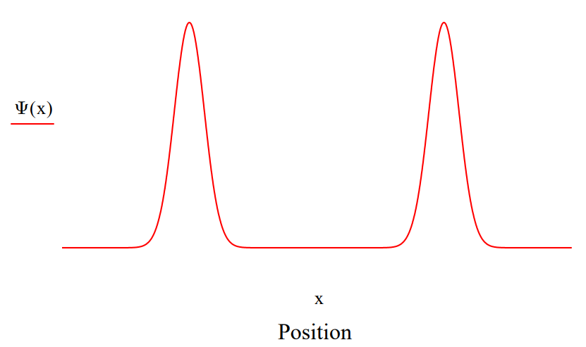
The coordinate wavefunction is Fourier transformed into momentum space to yield the diffraction pattern. Note that this calculation is in agreement with the well‐known double slit diffraction pattern.
\[
\Phi(p) :=\frac{1}{\sqrt{2 \cdot \pi}} \int_{-6}^{6} \exp (-\mathrm{i} \cdot p \cdot x) \cdot \Psi(x) d x
\nonumber \]
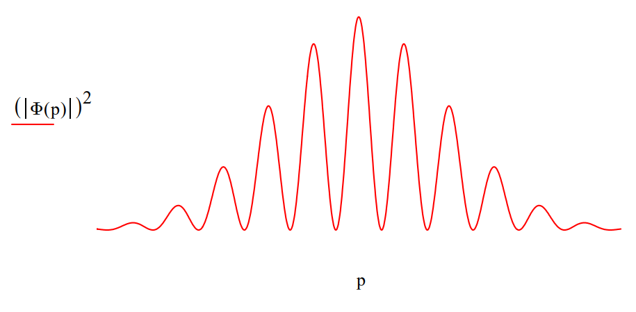
The Wigner function is a phase‐space distribution that is obtained by the Fourier transform of either the coordinate or momentum wavefunction. We use the coordinate wavefunction.
\[
\mathrm{W}(\mathrm{x}, \mathrm{p}) :=\frac{1}{\pi^{\frac{3}{2}}} \cdot \int_{-\infty}^{\infty} \Psi\left(\mathrm{x}+\frac{\mathrm{s}}{2}\right) \cdot \exp (\mathrm{i} \cdot \mathrm{s} \cdot \mathrm{p}) \cdot \Psi\left(\mathrm{x}-\frac{\mathrm{s}}{2}\right) \mathrm{ds}
\nonumber \]
\[
\mathrm{N} :=100 \qquad \mathrm{i} :=0 \ldots \mathrm{N} \qquad \mathrm{x}_{\mathrm{i}}=-4+\frac{8 \cdot \mathrm{i}}{\mathrm{N}} \\ \mathrm{j} :=0 \ldots \mathrm{N} \qquad \mathrm{p}_{\mathrm{j}}=-6+\frac{12 \cdot \mathrm{j}}{\mathrm{N}} \qquad \text{Wigner}_{\mathrm{i}, \mathrm{j}}:=\mathrm{W}\left(\mathrm{x}_{\mathrm{i}}, \mathrm{p}_{\mathrm{j}}\right)
\nonumber \]
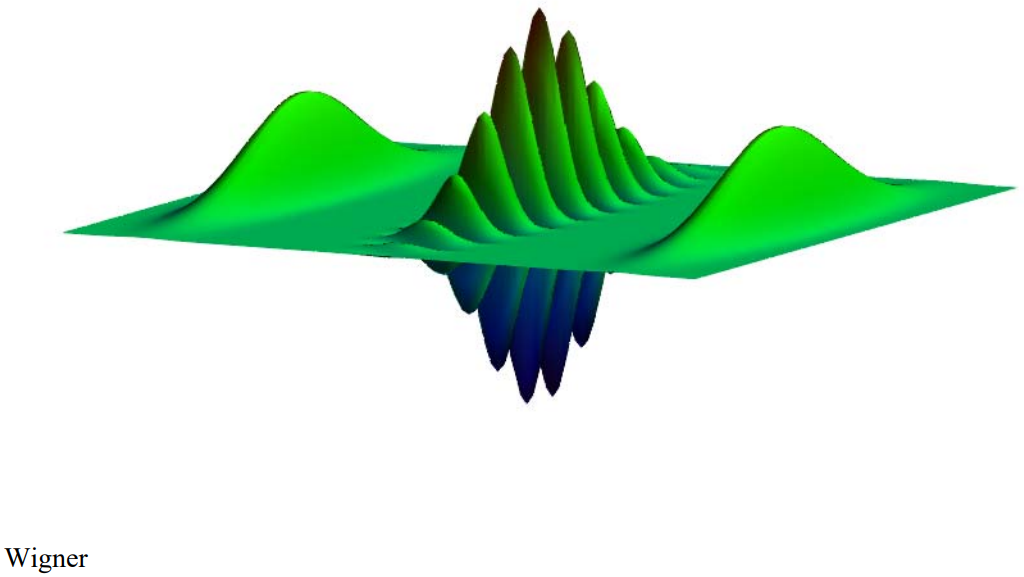
The Wigner distribution is frequently called a quasi‐probability distribution because, as can be seen in the display above, it can have negative values. Integration of the Wigner function with respect to momentum recovers the coordinate wavefunction and integration with respect to position yields the momentum wavefunction.
\[
\Psi_{\mathrm{w}}(\mathrm{x}) :=\int_{-6}^{6} \mathrm{W}(\mathrm{x}, \mathrm{p}) \text { dp } \quad \mathrm{x} :=-5,-4.98\ldots5 \\ \Phi_{\mathrm{w}}(\mathrm{p}) :=\int_{-5}^{5} \mathrm{W}(\mathrm{x}, \mathrm{p}) \mathrm{dx} \quad \mathrm{p} :=-6,-5.98\ldots6
\nonumber \]
The Wigner distribution can be reconstructed from experimental measurements using quantum state tomography. Reconstructive tomography is a widely used technique in medicine, for example, for obtaining the shape of an inaccessible two‐dimensional object from a set of different one‐dimensional ʺshadowsʺ cast by that object.
Quantum state reconstruction is possible if a system can be prepared repeatedly in the same state. Subsequent measurements on such a system are then effectively mutltiple measurements on the same quantum state. The theoretical Wigner distribution shown above for the double‐slit experiment has been reconstructed for the helium atom. [See, Nature, 386, 150 (1997).
See Figure 1 of ʺShadows and Mirrors:Reconstructing Quantum States of Atom Motion,ʺ Physics Today, April 1998, by Leibfried, Pfau, and Monroe.
Reference: Decoherence and the Transition form Quantum to Classical, Wojciech Jurek, Physics Today, October 1991, pages 36‐44.