1.20: The Repackaging of Quantum Weirdness

Quantum mechanics offers its students and practitioners several significant conceptual challenges, among them differential operators, wave-particle duality, tunneling, uncertainty, superpositions, interference, entanglement, and non-local correlations. This tutorial deals with just one of these challenges - the concept of the quantum mechanical operator and how it extracts information from the wavefunction. Professor Chris Cramer (University of Minnesota) likens the wavefunction to an oracle - it knows all and tells some when properly addressed and questioned.

According to Daniel F. Styer (Oberlin College) there are at least nine formulations of quantum mechanics. In this tutorial the position and momentum operators will be examined in the coordinate, momentum and phase space formulations of quantum mechanics. The table below lists the forms of the operators in each of these representations. Clearly the multiplicative character of the phase space operators appeals to our classical prejudices and intuition. The differential form of the momentum operator in coordinate space and position operator in momentum space are signatures of the weird and deeply non-classical character of quantum theory. However, as we shall see the quantum weirdness in the phase-space formulation has simply been temporarily hidden.

According to Styer [Amer. J. Phys. 70, 297 (2002)], "The various formulations package that weirdness in various ways, but none of them can eliminate it because the weirdness comes from the facts, not the formalism."

\[\begin{pmatrix} \text{Operator} & \text{CoordinateSpace} & \text{MomentumSpace} & \text{PhaseSpace} \\ \text{position} & x \cdot \Box & i \cdot \frac{d}{dp} \Box & x \cdot \Box \\ \text{momentum} & \frac{1}{i} \cdot \frac{d}{dx} \Box & p \cdot \Box & p \cdot \Box \end{pmatrix} \nonumber \]

The first excited state of the harmonic oscillator will be used to illustrate the repackaging of quantum weirdness. All calculations are carried out in atomic units (h = 2\(\pi\)), and in the interest of mathematical clarity and expediency we add the following restriction, \(\mu\) = k =1.

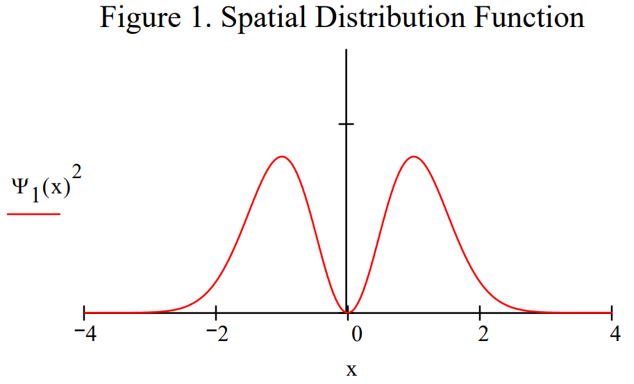
We begin in coordinate space by demonstrating that the \(v = 1\) wavefunction is normalized and displaying its spatial distribution function. Next we calculate the expectation value for the energy and demonstrate that the wavefunction is an eigenfunction of the energy operator.

Next the v = 1 spatial wavefunction is Fourier transformed into the momentum representation and everything done for the coordinate wavefunction is repeated. We get the same result for the energy calculation, as expected. We also find, also as expected, that the momentum wavefunction is also an eigenfunction of the energy operator. To prove that this is a two-way street, we Fourier transform the momentum wavefunction back to the coordinate representation.

In the last section the Wigner function, a phase-space (coordinate-momentum space) distribution function is generated from both the coordinate and momentum wavefunctions. The calculation for the energy has a classical look to it (both position and momentum are multiplicative operators) and the result agrees with the coordinate and momentum space calculations. However, it will be easy to show that the quantum weirdness has just been hidden from direct view.

Coordinate Representation

\[
\Psi_{1}(x) :=\left(\frac{4}{\pi}\right)^{\frac{1}{4}} \cdot x \cdot \exp \left(-\frac{x^{2}}{2}\right) \qquad \int_{-\infty}^{\infty} \Psi_{1}(x)^{2} d x=1
\nonumber \]

Energy expectation value:

\[
\int_{-\infty}^{\infty} \Psi_{1}(x) \cdot \frac{-1}{2} \cdot \frac{d^{2}}{d x^{2}} \Psi_{1}(x) d x+\int_{-\infty}^{\infty} \Psi_{1}(x) \cdot \frac{1}{2} \cdot x^{2} \cdot \Psi_{1}(x) d x=1.5
\nonumber \]

The wavefunction is an eigenfunction of the energy operator:

\[
\frac{-1}{2} \cdot \frac{\mathrm{d}^{2}}{\mathrm{dx}^{2}} \Psi_{1}(\mathrm{x})+\frac{1}{2} \cdot \mathrm{x}^{2} \cdot \Psi_{1}(\mathrm{x})=\mathrm{E} \cdot \Psi_{1}(\mathrm{x}) \text { solve }, \mathrm{E} \rightarrow \frac{3}{2}
\nonumber \]

Momentum Representation

A Fourier transform of the coordinate wavefunction yields the momentum space wavefunction.

\[
\Phi_{1}(\mathrm{p}) :=\frac{1}{\sqrt{2 \cdot \pi}} \cdot \int_{-\infty}^{\infty} \exp (-\mathrm{i} \cdot \mathrm{p} \cdot \mathrm{x}) \Psi_{1}(\mathrm{x}) \mathrm{d} \mathrm{x} \; \text{simplify} \rightarrow (-i) \cdot \frac{2^{\frac{1}{2}}}{\pi^{\frac{1}{4}}} \cdot \mathrm{e}^{\frac{-1}{2} \cdot \mathrm{p}^{2}} \cdot \mathrm{p}
\nonumber \]

\[
\int_{-\infty}^{\infty}\left(\left|\Phi_{1}(\mathrm{p})\right|\right)^{2} \mathrm{d} \mathrm{p}=1
\nonumber \]

Of course, a Fourier transform of the momentum wavefunction returns the coordinate wavefunction.

\[
\frac{1}{\sqrt{2 \cdot \pi}} \cdot \int_{-\infty}^{\infty} \exp (\mathrm{i} \cdot \mathrm{p} \cdot \mathrm{x}) \Phi_{1}(\mathrm{p}) \mathrm{dp} \; \text{simplify} \rightarrow \mathrm{e}^{\frac{-1}{2} \cdot \mathrm{x}^{2}} \cdot \frac{2^{\frac{1}{2}}}{\pi^{\frac{1}{4}}} \cdot \mathrm{x}
\nonumber \]

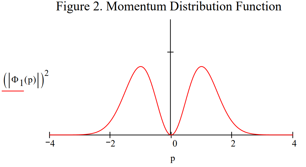
The momentum distribution is displayed and the energy calculations executed.

\[
\int_{-\infty}^{\infty} \overline{\Phi_{1}(p)} \cdot \frac{p^{2}}{2} \cdot \Phi_{1}(p) d p+\int_{-\infty}^{\infty} \overline{\Phi_{1}(p)} \cdot \frac{-1}{2} \cdot \frac{d^{2}}{d p^{2}} \Phi_{1}(p) d p=1.5
\nonumber \]

\[
\frac{\mathrm{p}^{2}}{2} \cdot \Phi_{1}(\mathrm{p})+\frac{-1}{2} \cdot \frac{\mathrm{d}^{2}}{\mathrm{d} \mathrm{p}^{2}} \Phi_{1}(\mathrm{p})=\mathrm{E} \cdot \Phi_{1}(\mathrm{p}) \text { solve }, \mathrm{E} \rightarrow \frac{3}{2}
\nonumber \]

Phase Space Representation

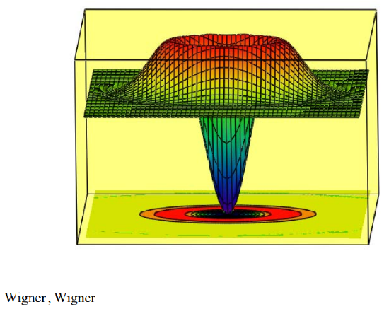
As shown below, the Wigner phase-space distribution function can be generated from either the coordinate or momentum wavefunctions. A deconstruction of the Wigner function can be found at: http://www.users.csbsju.edu/~frioux/wigner/wigner.pdf.

\[
\mathrm{W}_{1}(\mathrm{x}, \mathrm{p}) :=\frac{1}{2 \pi} \cdot \int_{-\infty}^{\infty} \exp (\mathrm{i} \cdot \mathrm{s} \cdot \mathrm{p}) \cdot \Psi_{1}\left(\mathrm{x}+\frac{\mathrm{s}}{2}\right) \cdot \Psi_{1}\left(\mathrm{x}-\frac{\mathrm{s}}{2}\right) \mathrm{ds} \; \text{simplify} \\ \rightarrow \mathrm{e}^{\left(-\mathrm{x}^{2}\right)-\mathrm{p}^{2}} \cdot \frac{2 \cdot \mathrm{x}^{2}+2 \cdot \mathrm{p}^{2}-1}{\pi}
\nonumber \]

\[
\frac{1}{2 \pi} \cdot \int_{-\infty}^{\infty} \exp (\mathrm{i} \cdot \mathrm{s} \cdot \mathrm{x}) \cdot \Phi_{1}\left(\mathrm{p}+\frac{\mathrm{s}}{2}\right) \cdot \Phi_{1}\left(\mathrm{p}-\frac{\mathrm{s}}{2}\right) \mathrm{ds} \; \text{simplify} \\ \rightarrow -\mathrm{e}^{\left(-\mathrm{x}^{2}\right)-\mathrm{p}^{2}} \cdot \frac{2 \cdot \mathrm{x}^{2}+2 \cdot \mathrm{p}^{2}-1}{\pi}
\nonumber \]

Integration over the spatial and momentum coordinates shows that the Wigner function is normalized.

\[
\int_{-\infty}^{\infty} \int_{-\infty}^{\infty} W_{1}(x, p) d x d p=1
\nonumber \]

Integration over the momentum coordinate yields the spatial distribution function, exactly the same as graphed in Figure 1.

\[
\int_{-\infty}^{\infty} \mathrm{W}_{1}(\mathrm{x}, \mathrm{p}) \text { dp simplify } \rightarrow 2 \cdot \mathrm{e}^{-\mathrm{x}^{2}} \cdot \frac{\mathrm{x}^{2}}{\pi^{\frac{1}{2}}}
\nonumber \]

Integration over the spatial coordinate yields the momentum distribution function, exactly the same as graphed in Figure 2.

\[
\int_{-\infty}^{\infty} \mathrm{W}_{1}(\mathrm{x}, \mathrm{p}) \mathrm{dx} \text { simplify } \rightarrow 2 \cdot \mathrm{e}^{-\mathrm{p}^{2}} \cdot \frac{\mathrm{p}^{2}}{\pi^{\frac{1}{2}}}
\nonumber \]

The expectation value for the total energy using the Wigner distribution is the same as that obtained previously with the coordinate and momentum wavefunctions.

\[
\int_{-\infty}^{\infty} \int_{-\infty}^{\infty}\left(\frac{p^{2}}{2}+\frac{x^{2}}{2}\right) \cdot W_{1}(x, p) d x d p=1.5
\nonumber \]

This calculation has true classical flavor. The energy values, which are a function of x and p, are weighted by the phase-space (p-x) distribution function, followed by integration over all possible values of position and momentum. That quantum weirdness is being hidden is revealed when the Wigner distribution function is graphed. It can have negative values and therefore can't be a true probability distribution function. For this reason the Wigner function is referred to as a quasi-probability distribution function. In summary, in order to recover a classical-like energy calculation in quantum mechanics one has to be able to tolerate negative probabilities!

\[
\mathrm{N} :=60 \qquad \mathrm{i} :=0 \ldots \mathrm{N} \qquad \mathrm{x}_{\mathrm{i}} :=-3+\frac{6 \cdot \mathrm{i}}{\mathrm{N}} \qquad \mathrm{j} :=0 \ldots \mathrm{N} \qquad \mathrm{p}_{\mathrm{j}} :=-5+\frac{10 \cdot \mathrm{j}}{\mathrm{N}} \qquad \text { Wigner }_{\mathrm{i}, \mathrm{j}} :=\mathrm{W}_{1}\left(\mathrm{x}_{\mathrm{i}}, \mathrm{p}_{\mathrm{j}}\right)
\nonumber \]