1.15: Quantum Mechanics and the Fourier Transform

Quantum chemists work almost exclusively in coordinate space because they need wave functions that will help them understand molecular structure and chemical reactivity. They need the location of the nuclear centers and electron density maps. Consequently undergraduate physical chemistry texts examine all the traditional model problems (particle in a box, rigid rotor, harmonic oscillator, hydrogen atom, hydrogen molecule ion, hydrogen molecule, etc.) using spatial wave functions. Students learn how to interpret graphical representations of the various wave functions. If knowledge is required about electron momentum, for example, expectation values are calculated using the coordinate wave function.

For the model systems listed above, it is a simple matter to carry out a Fourier transform into momentum space. This allows the same kind of visualization in momentum space that is available in the coordinate representation. The value of this capability in presenting a graphical illustration of the uncertainty principle for the particle-in-the-box (PIB) problem is illustrated in the following tutorial.

A Graphical Illustration of the Heisenberg Uncertainty Relationship

According to quantum mechanics position and momentum are conjugate variables; they cannot be simultaneously known with high precision. The uncertainty principle requires that if the position of an object is precisely known, its momentum is uncertain, and vice versa. This reciprocal relationship is captured by the well-known uncertainty relation, which says that the product of the uncertainties in position and momentum must be greater than or equal to Planck's constant divided by 4\(\pi\).

\[
\Delta x \cdot \Delta p \geq \frac{h}{4 \cdot \pi}
\nonumber \]

This simple mathematical relation can be visualized using the traditional work horse - the quantum mechanical particle in a box (infinite one-dimensional potential well). The particle's ground-state wave function in coordinate space for a box of width a is shown below.

\[
\Psi(\mathrm{x}, \mathrm{a}) :=\sqrt{\frac{2}{\mathrm{a}}} \cdot \sin \left(\frac{\pi \cdot \mathrm{x}}{\mathrm{a}}\right)
\nonumber \]

To illustrate the uncertainty principle and the reciprocal relationship between position and momentum, \(\Psi\)(x,a) is Fourier transformed into momentum space yielding the particle's ground-atate wave function in the momentum representation.

\[
\Phi(p, a) :=\sqrt{\frac{1}{2 \cdot \pi}} \cdot \int_{0}^{a} \exp (-i \cdot p \cdot x) \cdot \sqrt{\frac{2}{a}} \cdot \sin \left(\frac{\pi \cdot x}{a}\right) d x \operatorname{simplify} \rightarrow \frac{\pi \cdot a \cdot\left(e^{-a \cdot p \cdot 1}+1\right) \cdot \sqrt{\frac{1}{a}}}{\pi^{\frac{5}{2}}-\sqrt{\pi} \cdot a^{2} \cdot p^{2}}
\nonumber \]

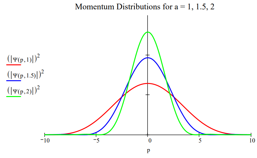
In the figure below, the momentum distribution, \(|\Phi(p, a)|^{2}\), is shown for three sizes, a = 1,2 and 3. The uncertainty principle is illustrated as follows: as the box size increases the position uncertainty increases and momentum uncertainty decreases because the momentum distribution narrows.

We use the particle-in-the-box example to introduce students to almost all the fundamental quantum mechanical concepts. When we come to spectroscopy and the chemical bond, we initially model the chemical bond as a harmonic oscillator. Here there are two physical parameters, force constant and effective mass. The following tutorial shows how the coordinate and momentum wave functions can be used to illustrate the uncertainty principle for various values of k and \(\mu\).

The Harmonic Oscillator and the Uncertainty Principle

Schrödinger's equation in atomic units (h = 2\(\pi\)) for the harmonic oscillator has an exact analytical solution.

\[
\mathrm{V}(\mathrm{x}, \mathrm{k}) :=\frac{1}{2} \cdot \mathrm{k} \cdot \mathrm{x}^{2} \quad \frac{-1}{2 \cdot \mu} \cdot \frac{\mathrm{d}^{2}}{\mathrm{dx}^{2}} \Psi(\mathrm{x})+\mathrm{V}(\mathrm{x}) \cdot \Psi(\mathrm{x})=\mathrm{E} \cdot \Psi(\mathrm{x})
\nonumber \]

The ground-state wave function (coordinate space) and energy for an oscillator with reduced mass \(\mu\) and force constant k are as follows.

\[
\Psi(\mathrm{x}, \mathrm{k}, \mu) :=\left(\frac{\sqrt{\mathrm{k} \cdot \mu}}{\pi}\right)^{\frac{1}{4}} \cdot \exp \left(-\sqrt{\mathrm{k} \cdot \mu} \cdot \frac{\mathrm{x}^{2}}{2}\right) \quad \mathrm{E}(\mathrm{k}, \mu) :=\frac{1}{2} \cdot \sqrt{\frac{\mathrm{k}}{\mu}}
\nonumber \]

The first thing we want to illustrate is that tunneling occurs in the simple harmonic oscillator. The classical turning point is that position at which the total energy is equal to the potential energy. In other words, classically the kinetic energy is zero and the oscillator's direction is going to reverse. For the ground state the classical turning point is,

\[
\frac{1}{2} \cdot \sqrt{\frac{\mathrm{k}}{\mu}}=\frac{1}{2} \cdot \mathrm{k} \cdot \mathrm{x}^{2} \text { has solution }(\mathrm{s}) \left( \begin{array}{c}{\frac{-1}{k^{\frac{1}{4}}\cdot \mu^{\frac{1}{4}}}} \\ {\frac{1}{k^{\frac{1}{4}} \cdot \mu^{\frac{1}{4}}}} \end{array}\right)
\nonumber \]

From the quantum mechanical perspective the oscillator is not vibrating; it is in a stationary state. To the extent that the oscillator's wave function extends beyond the classical turning point, tunneling is occurring. The calculation below shows that the probability that tunneling occurs is independent of the values of k and \(\mu\) for the ground state.

\[
2 \cdot\left[\int_\frac{1}{(\mathrm{k} \cdot \mu)^{\frac{1}{4}}}^{\infty}\left[\left(\frac{\sqrt{\mathrm{k} \cdot \mu}}{\pi}\right)^{\frac{1}{4}} \cdot \exp \left(-\sqrt{\mathrm{k} \cdot \mu} \cdot \frac{\mathrm{x}^{2}}{2}\right)\right]^{2} \mathrm{dx}\right] \Bigg|^{\text { assume, k> } 0, \mu>0}_{ \text { simplify }} \rightarrow 1-\operatorname{erf}(1)=0.157
\nonumber \]

A Fourier transform of the coordinate wave function provides its counter part in momentum space.

\[
\Phi(\mathbf{p}, \mathbf{k}, \boldsymbol{\mu}) :=\frac{1}{\sqrt{2 \cdot \pi}} \cdot \int_{-\infty}^{\infty} \exp (-\mathbf{i} \cdot \mathbf{p} \cdot \mathbf{x}) \cdot \Psi(\mathbf{x}, \mathbf{k}, \boldsymbol{\mu}) \mathrm{d} \mathbf{x} \Bigg| \begin{array}{l}{\text { assume, } \mathrm{k}>0} \\ {\text { assume, } \mu>0} \\ {\text { simplify }}\end{array}\rightarrow \frac{e^{-\frac{p^{2}}{2 \cdot \sqrt{\mu} \cdot \sqrt{k}}}}{\pi^{\frac{1}{4}} \cdot \mu^{\frac{1}{8}} \cdot k^{\frac{1}{8}}}
\nonumber \]

The uncertainty principle can now be illustrated by comparing the coordinate and momentum wave functions for a variety values of k and \(\mu\). For the benchmark case, k = \(\mu\) = 1, we see that the coordinate and momentum wave functions are identical and the classical turning point (CTP) is 1. The classical turning point will be taken as a measure of the spatial domain of the oscillator.

• For k = 2 and \(\mu\) =1, the force constant has doubled reducing the amplitude of vibration (CTP =0.841) and therefore the uncertainty in position. Consequently there is an increase in the uncertainty in momentum which is manifested by a broader momentum distribution function.
• For k = 1 and \(\mu\) = 2, the increase in effective mass drops the oscillator in the potential well decreasing the vibrational amplitude (CTP = 0.841) causing a decrease in \(\Delta\)x and an increase in \(\Delta\)p.
• For k = 0.5 and \(\mu\) = 1, the lower force constant causes a larger vibrational amplitude (CTP = 1.189) and an accompanying increase in \(\Delta\)x. Consequently \(\Delta\)p decreases.

Force constant: \(k := 0.5\)

Effective mass: \(\mu := 1\)

Energy: \(\mathrm{E}(\mathrm{k}, \mu)=0.354\)

CTP: \(\frac{1}{\mathrm{k}^{\frac{1}{4}} \cdot \mu^{\frac{1}{4}}}=1.189\)

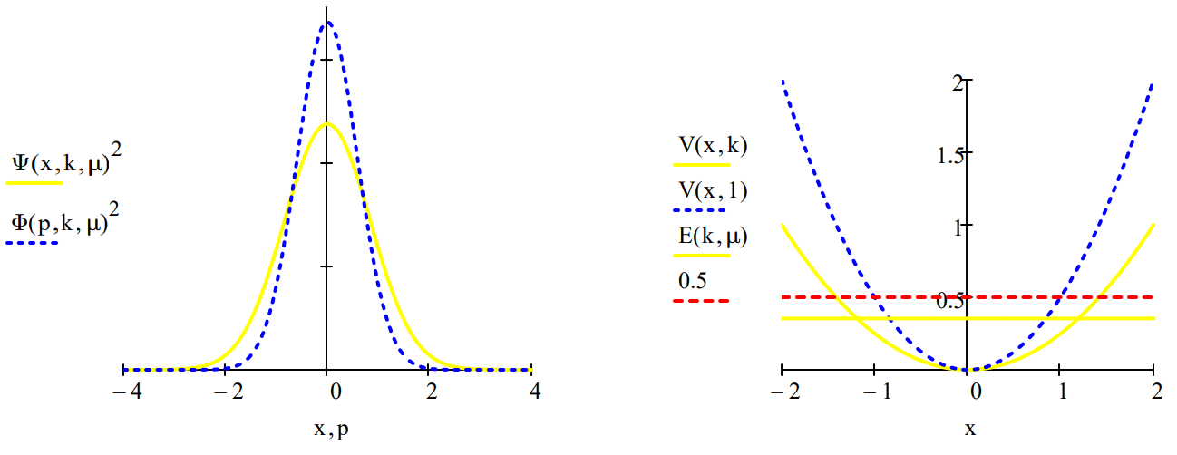
The uncertainties in position and momentum are calculated as shown below because for the harmonic oscillator \(<x>=

=0\).

\[
\Delta x :=\sqrt{\int_{-\infty}^{\infty} x^{2} \cdot \Psi(x, k, \mu)^{2} d x}=0.841 \quad \Delta \mathrm{p} :=\sqrt{\int_{-\infty}^{\infty} \mathrm{p}^{2} \cdot \Phi(\mathrm{p}, \mathrm{k}, \mu)^{2} \mathrm{d} \mathrm{p}=0.595} \quad \Delta x \cdot \Delta p=0.5
\nonumber \]

A summary of the four cases considered is provided in the table below.

\[
\left( \begin{array}{cccccc}{\mu} & {k} & {C T P} & {\Delta x} & {\Delta p} & {\Delta x \Delta p} \\ {1} & {1} & {1.00} & {0.707} & {0.707} & {0.5} \\ {1} & {2} & {0.841} & {0.595} & {0.841} & {0.5} \\ {2} & {1} & {0.841} & {0.595} & {0.841} & {0.5} \\ {1} & {0.5} & {1.189} & {0.841} & {0.594} & {0.5}\end{array}\right)
\nonumber \]

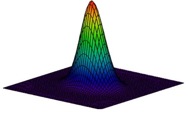
The Wigner function, W(x,p), is a phase-space distribution that can be used to provide an alternative graphical representation of the results calculated above. As shown below it can be generated using either the coordinate or momentum wave function.

Calculate Wigner distribution:

\[
\mathrm{W}(\mathrm{x}, \mathrm{p}) :=\frac{1}{\pi^{\frac{3}{2}}} \cdot \int_{-\infty}^{\infty} \Psi\left(\mathrm{x}+\frac{\mathrm{s}}{2}, \mathrm{k}, \mu\right) \cdot \exp (\mathrm{i} \cdot \mathrm{s} \cdot \mathrm{p}) \cdot \Psi\left(\mathrm{x}-\frac{\mathrm{s}}{2}, \mathrm{k}, \mu\right) \mathrm{ds}
\nonumber \]

Display Wigner distribution:

\[
\mathrm{N} :=50 \quad \mathrm{i} :=0 \ldots \mathrm{N} \quad \mathrm{x}_{\mathrm{i}} :=-4+\frac{8 \cdot \mathrm{i}}{\mathrm{N}} \quad \mathrm{j} :=0 \ldots \mathrm{N} \quad \mathrm{p}_{\mathrm{j}} :=-4+\frac{8 \cdot \mathrm{j}}{\mathrm{N}} \quad \text { Wigner}_{\mathrm{i}, \mathrm{j}}=\mathrm{W}\left(\mathrm{x}_{\mathrm{i}}, \mathrm{p}_{\mathrm{j}}\right)
\nonumber \]

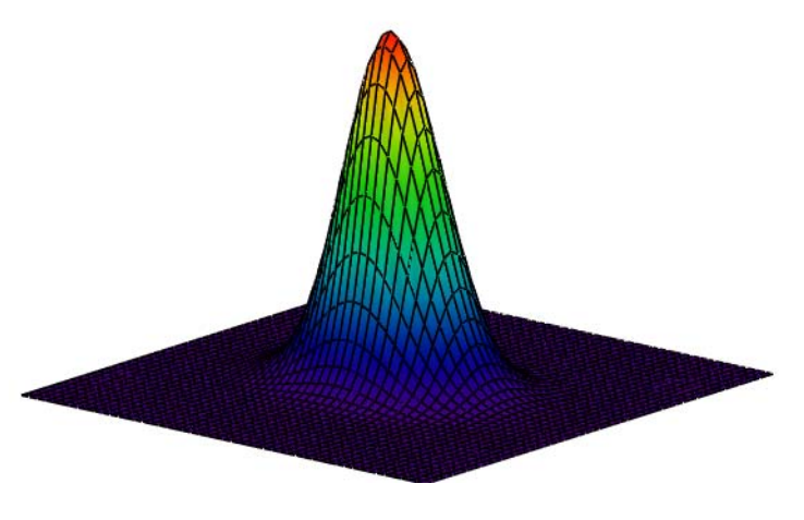
Calculate Wigner distribution:

\[
\mathrm{W}(\mathrm{x}, \mathrm{p}) :=\frac{1}{\pi^{\frac{3}{2}}} \cdot \int_{-\infty}^{\infty} \Phi\left(\mathrm{p}+\frac{\mathrm{s}}{2}, \mathrm{k}, \mu\right) \cdot \exp (\mathrm{i} \cdot \mathrm{s} \cdot \mathrm{x}) \cdot \Phi\left(\mathrm{p}-\frac{\mathrm{s}}{2}, \mathrm{k}, \mu\right) \mathrm{ds}
\nonumber \]

Display Wigner distribution:

\[
\mathrm{N} :=50 \quad \mathrm{i} :=0 \ldots \mathrm{N} \quad \mathrm{x}_{\mathrm{i}} :=-4+\frac{8 \cdot \mathrm{i}}{\mathrm{N}} \quad \mathbf{j} :=0 \ldots \mathrm{N} \quad \mathrm{p}_{\mathrm{j}} :=-4+\frac{8 \cdot \mathrm{j}}{\mathrm{N}} \quad \text { Wigner}_{\mathrm{i}, \mathrm{j}} :=\mathrm{W}\left(\mathrm{x}_{\mathrm{i}}, \mathrm{p}_{\mathrm{j}}\right)
\nonumber \]

It is easy to derive the angular position, angular momentum uncertainty relationship for a particle on a ring using the position-momentum uncertainty equation and the classical definition of angular momentum. Visualization is provided by the next tutorial.

Demonstrating the Uncertainty Principle for Angular Momentum and Angular Position

The uncertainty relation between angular momentum and angular position can be derived from the more familiar uncertainty relation between linear momentum and position

\[
\Delta \mathrm{p} \cdot \Delta \mathrm{x} \geq \frac{\mathrm{h}}{4 \cdot \pi} \tag{1}
\nonumber \]

Consider a particle with linear momentum p moving on a circle of radius r. The particleʹs angular momentum is given by equation (2).

\[
\mathrm{L}=\mathrm{m} \cdot \mathrm{v} \cdot \mathrm{r}=\mathrm{p} \cdot \mathrm{r} \tag{2}
\nonumber \]

In moving a distance x on the circle the particle sweeps out an angle \(\phi\) in radians.

\[
\phi=\frac{x}{r} \tag{3}
\nonumber \]

Equations (2) and (3) suggest,

\[
\Delta \mathrm{p}=\frac{\Delta \mathrm{L}}{\mathrm{r}} \qquad \Delta \mathrm{x}=\Delta \phi \cdot \mathrm{r} \tag{4}
\nonumber \]

Substitution of equations (4) into equation (1) yields the angular momentum, angular position uncertainty relation.

\[
\Delta \mathrm{L} \cdot \Delta \phi \geq \frac{\mathrm{h}}{4 \cdot \pi} \tag{5}
\nonumber \]

In addition to the Heisenberg restrictions represented by equations (1) and (5), conjugate observables are related by Fourier transforms. For example, for position and momentum it is given by equation (6) in atomic units (h = 2\(\pi\)).

\[
\langle p | x\rangle=\frac{1}{\sqrt{2 \pi}} \exp (-i p x) \tag{6}
\nonumber \]

Equations (2) and (3) can be used with (6) to obtain the Fourier transform between angular momentum and angular position.

\[
\langle L | \phi\rangle=\frac{1}{\sqrt{2 \pi}} \exp (-i L \phi) \tag{7}
\nonumber \]

Equations (6) and (7) are mathematical dictionaries telling us how to translate from x language to p language, or \(\phi\) language to L language. The complex conjugates of (6) and (7) translate in the reverse direction, from p to x and from L to \(\phi\).

The work‐horse particle‐in‐a‐box (PIB) problem can be used to provide a compelling graphical illustration of the position‐momentum uncertainty relation. The position wave function for the ground state of a PIB in a box of length a is given below.

\[
\langle x | \Psi\rangle=\sqrt{\frac{2}{a}} \sin \left(\frac{\pi x}{a}\right) \tag{8}
\nonumber \]

The conjugate momentum‐space wave function is obtained by the following Fourier transform.

\[
\langle p | \Psi\rangle=\int_{0}^{a}\langle p | x\rangle\langle x | \Psi\rangle d x=\frac{1}{\sqrt{\pi a}} \int_{0}^{a} \exp (-i p x) \sin \left(\frac{\pi x}{a}\right) \tag{9}
\nonumber \]

Evaluation of the integral in equation (9) yields

\[
\Psi(\mathrm{p}, \mathrm{a}) :=\sqrt{\mathrm{a} \cdot \pi} \cdot \frac{\exp (-\mathrm{i} \cdot \mathrm{p} \cdot \mathrm{a})+1}{\pi^{2}-\mathrm{p}^{2} \cdot \mathrm{a}^{2}} \tag{10}
\nonumber \]

Plotting the momentum distribution function for several box lengths, as is done in the figure below, clearly reveals the position‐momentum uncertainty relation. The greater the box length the greater the uncertainty in position. However, as the figure shows, the greater the box length the narrower the momentum distribution, and, consequently, the smaller the uncertainty in momentum.

A similar visualization of the angular‐momentum/angular‐position uncertainty relation is also possible. Suppose a particle on a ring is prepared in such a way that its angular wave function is represented by the following gaussian function,

\[
\langle\phi | \Psi\rangle=\exp \left(-a \phi^{2}\right) \tag{11}
\nonumber \]

where the parameter a controls the width of the angular distribution. The conjugate angular momentum wave function is obtained by the following Fourier transform.

\[
\langle L | \Psi\rangle=\int_{-\pi}^{\pi}\langle L | \phi\rangle\langle\phi | \Psi\rangle d \phi=\frac{1}{\sqrt{2 \pi}} \int_{-\pi}^{\pi} \exp (-i L \phi) \exp \left(-a \phi^{2}\right) d \phi \tag{12}
\nonumber \]

Plots of \(|<\phi| \Psi>\left.\right|^{2}\) and \(|<L| \Psi>\left.\right|^{2}\) shown below for two values of the parameter a illustrate the angular momentum/angular position uncertainty relation. The larger the value of a, the smaller the angular positional uncertainty and the greater the angular momentum uncertainty. In other words, the greater the value of a the greater the number of angular momentum eigenstates observed.

\[
\mathrm{a} :=0.5 \qquad \Phi(\phi, \mathrm{a}) :=\exp \left(-\mathrm{a} \cdot \phi^{2}\right)
\nonumber \]

\[
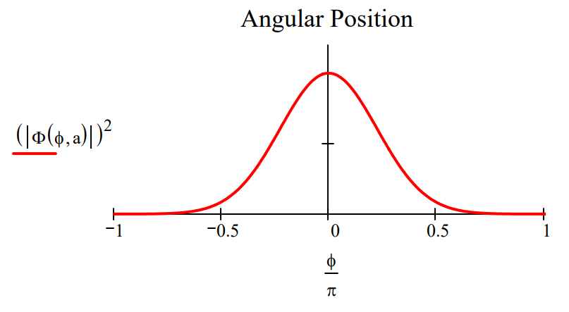
\mathrm{L} :=-5 \ldots5 \qquad \Psi(\mathrm{L}, \mathrm{a}) :=\int_{-\pi}^{\pi} \exp (-\mathrm{i} \cdot \mathrm{L} \cdot \phi) \Phi(\phi, \mathrm{a}) \mathrm{d} \phi
\nonumber \]

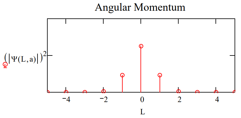
Make the angular position distribution narrower: \(a : = 2.5\)

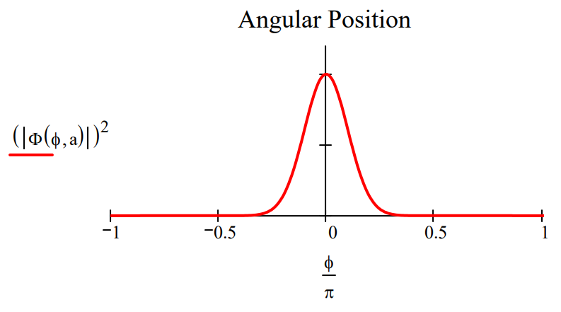
Observe a broader distribution in angular momentum.

The uncertainty relation between angular position and angular momentum as outlined above is a simplified version of that presented by S. Franke‐Arnold et al. in New Journal of Physics 6, 103 (2004).