1.14: Quantum Mechanics and the Fourier Transform

However, just as with the circular aperture (Airy pattern) a single slit also yields a diffraction pattern when illuminated. Both are examples of the superposition principle because the photons that arrive at the detection screen can get there from any points within the aperture or slit. So, in general, we calculate the diffraction pattern by a Fourier transform of the coordinate space geometry, slit or circle or something more complicated. The following tutorial explores single-slit diffraction and the uncertainty principle.

A Quantum Mechanical Interpretation of Single‐slit Diffraction

Diffraction has a simple quantum mechanical interpretation based on the uncertainty principle. Or we could say diffraction is an excellent way to illustrate the uncertainty principle.

A screen with a single slit of width, w, is illuminated with a coherent photon or particle beam. The normalized coordinate‐space wave function at the slit screen is,

\[
\mathrm{w} :=1 \qquad \Psi(\mathrm{x}, \mathrm{w}) :=\mathrm{if}\left[\left(\mathrm{x} \geq-\frac{\mathrm{w}}{2}\right) \cdot\left(\mathrm{x} \leq \frac{\mathrm{w}}{2}\right), \frac{1}{\sqrt{\mathrm{w}}}, 0\right] \qquad \mathrm{x} :=\frac{-\mathrm{w}}{2}, \frac{-\mathrm{w}}{2}+0.005 \ldots \frac{\mathrm{w}}{2}
\nonumber \]

The coordinate‐space probability density, \(|\Psi(x, w)|^{2}\), is displayed for a slit of unit width below

The slit‐screen measures position, it localizes the incident beam in the x‐direction. According to the uncertainty principle, because position and momentum are complementary, or conjugate, observables, this measurement must be accompanied by a delocalization of the x‐component of the momentum. This can be seen by a Fourier transform of \(\Psi (x,w)\) into momentum space to obtain the momentum wave function, \(\Phi (p_{x},w)\).

\[
\Phi\left(\mathrm{p}_{\mathrm{x}}, \mathrm{w}\right) :=\frac{1}{\sqrt{2 \cdot \pi}} \cdot \int_{-\frac{\mathrm{w}}{2}}^{\frac{\mathrm{w}}{2}} \exp \left(-\mathrm{i} \cdot \mathrm{p}_{\mathrm{x}} \cdot \mathrm{x}\right) \cdot \frac{1}{\sqrt{\mathrm{w}}} \mathrm{dx} \text { simplify } \rightarrow \frac{\sqrt{2} \cdot \sin \left(\frac{\mathrm{p}_{\mathrm{x}} \cdot \mathrm{w}}{2}\right)}{\sqrt{\pi} \cdot \mathrm{p}_{\mathrm{x}} \cdot \sqrt{\mathrm{w}}}
\nonumber \]

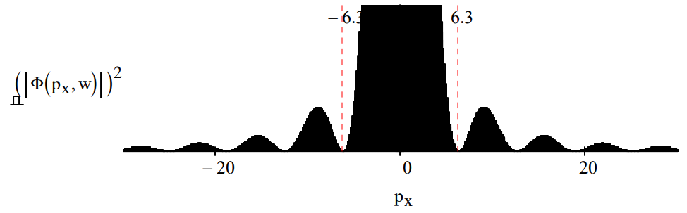
It is the momentum distribution, \(|\Phi(p_{x} ,w)|^{2}\), shown histographically below that is projected onto the detection screen. Thus, a position measurement at the detection screen is also effectively a measure of the x‐component of the particle momentum.

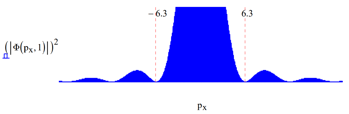
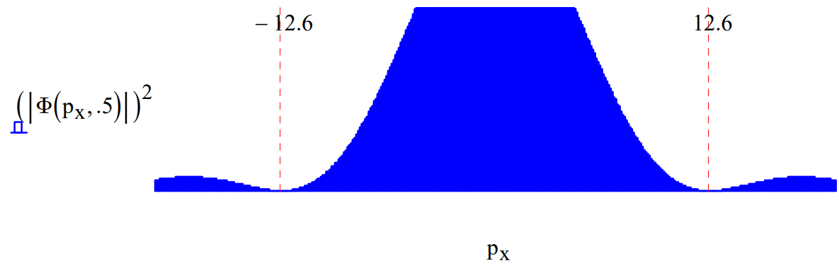
In this figure we see the spread in momentum required by the uncertainty principle, plus interference fringes due to the fact that the incident beam can imerge from any where within the slit, allowing for constructive and destructive interference at the detection screen. If the slit width is decreased the position is more precisely known and the uncertainty principle demands a broadening in the momentum distribution as shown below.

Equating uncertainty in position with slit width and uncertainty in momentum with the width of the intense center of the diffraction pattern, we have in atomic units: \(\Delta x \Delta p_{x}=12.6\). If the slit width is decreased the position is more precisely known and the uncertainty principle demands a broadening in the momentum distribution as shown below. For slit width 0.5 we again find the product of the uncertainties is 12.6.

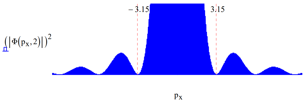
Naturally if the slit width is increased to 2.0 the position uncertainty increases and the uncertainty in momentum decreases yielding again \(\Delta x \Delta p_{x}=12.6\).

The x‐direction momentum can be expressed in terms of the wavelength of the illuminating beam and the diffraction angle using the following sequence of equations of which the second is the de Broglie relation in atomic units (h = 2\(\pi\)).

\[
\mathrm{p}_{\mathrm{x}}=\mathrm{p} \cdot \sin (\Theta) \qquad \mathrm{p}=\frac{2 \cdot \pi}{\lambda} \qquad \mathrm{p}_{\mathrm{x}}=\frac{2 \cdot \pi}{\lambda} \cdot \sin (\Theta)
\nonumber \]

\[
\Phi\left(\Theta_{\mathrm{x}}, \mathrm{w}, \lambda\right) :=\sqrt{\frac{2}{\pi \cdot \mathrm{w}} \cdot} \cdot \frac{\sin \left(\frac{\pi \cdot \mathrm{w}}{\lambda} \cdot \sin \left(\Theta_{\mathrm{x}}\right)\right)}{\frac{2 \cdot \pi}{\lambda} \cdot \sin \left(\Theta_{\mathrm{x}}\right)}
\nonumber \]

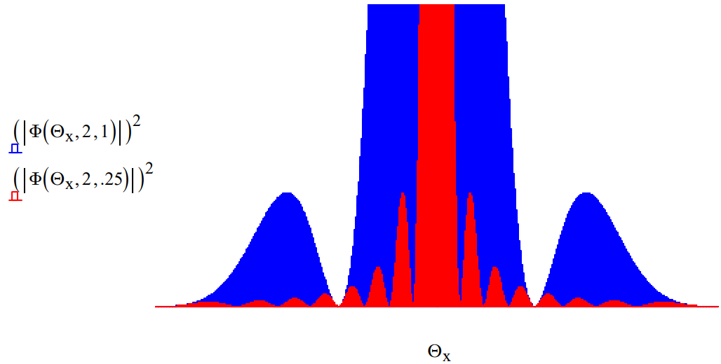
This allows one to explore the effect of the wavelength of the illuminating beam on the diffraction pattern. The figure below shows that a short wavelength (high momentum) illuminating beam gives rise to a narrower diffraction pattern.

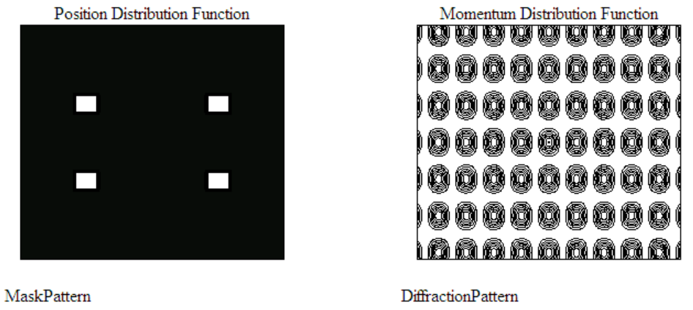
The method used here to calculate single‐slit diffraction patterns (momentum‐space distribution functions) is easily extended to multiple slits, and also to diffraction at two‐dimensional masks with a variety of hole geometries.

Relevant Literature:

Primary source: ʺQuantum interference with slits,ʺ Thomas Marcella which appeared in European Journal of Physics 23, 615‐621 (2002).

See also: ʺCalculating diffraction patterns,ʺ F. Rioux in European Journal of Physics, 24, N1‐N3 (2003). “Using Optical Transforms to Teach Quantum Mechanics,” F. Rioux; B. J. Johnson, The Chemical Educator, 9, 12‐16 (2004). ʺSingle‐slit Diffraction and the Uncertainty Prinicple,ʺ F. Rioux in Journal of Chemical Education, 82, 1210 (2005).

ʺExperimental verification of the Heisenberg uncertainty principle for hot fullerene moleculesʺ, O. Nairz, M. Arndt, and A. Zeilinger, Phys. Rev. A, 65, 032109 (2002).

ʺIntroducing the Uncertainty Principle Using Diffraction of Light Waves,ʺ Pedro L. Muino, Journal of Chemical Education, 77, 1025‐1027 (2000).

The next link shows how the methods used to examine these relatively simple cases can be expanded to more interesting geometries, including the DNA double helix. The following tutorial provides details regarding a simple simulation of the DNA diffraction pattern.

Simulating the DNA Diffraction Pattern

The publication of the DNA double-helix structure by x-ray diffraction in 1953 is one the most significant scientific events of the 20th century (1). Therefore, it is important that science students and their teachers have some understanding of how this great achievement was accomplished. X-ray diffraction is conceptually simple: a source of X-rays illuminates a sample which scatters the x-rays, and a detector records the arrival of the scattered x-rays (diffraction pattern). However, the mathematical analysis required to extract from diffraction pattern the molecular geometry of the sample that caused the diffraction pattern is quite formidable. Therefore, the purpose of this tutorial is to illustrate some of the elements of the mathematical analysis required to solve a structure.

The famous X-ray diffraction pattern obtained by Rosalind Franklin is shown below (2).

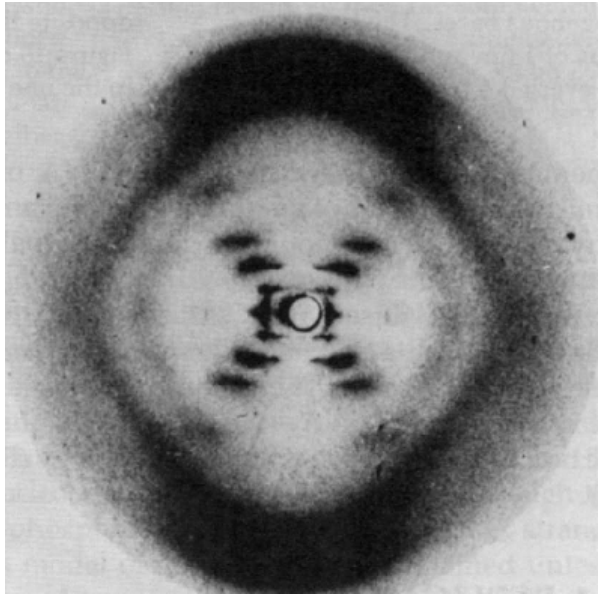
This X-ray picture stimulated Watson and Crick to propose the now famous double-helix sturcture for DNA. It was surely fortuitous that Crick had recently completed an unrelated study of the diffraction patterns of helical molecules ( 3).

To gain some understanding of how the experimental pattern led to the hypothesis of a double-helical structure we will work in reverse. We will assume the double-helix structure, calculate the diffraction pattern, and compare it with the experimental result. This, therefore, is a deductive exercise as opposed to the brilliant inductive accomplishment of Watson and Crick in determining the DNA structure from Franklin's experimental X-ray pattern.

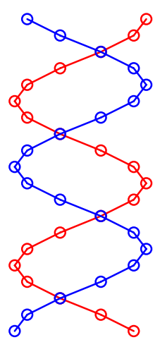
The experimental pattern will be simulated by modeling DNA solely as a planar double strand of sugar-phosphate backbone groups shown below. Reference 4 provides the justification and the limitations in using two-dimensional models for three-dimensional structures when simulating X-ray diffraction experiments.

The double-strand geometry shown below was created using the following mathematics. Calculations are carried out in atomic units.

Sugar-phosphate groups per strand: \(A : = 20\)

Strand radius: \(R : = 1\)

Phase difference between strands: \(0.8 \cdot \pi\)

First strand:

\[
\mathrm{m} :=1 \ldots \mathrm{A} \quad \Theta_{\mathrm{m}} :=\frac{4 \cdot \pi \cdot \mathrm{m}}{\mathrm{A}} \quad \mathrm{y}_{\mathrm{m}} :=\mathrm{m} \quad \mathrm{x}_{\mathrm{m}} :=\mathrm{R} \cdot \cos \left(\Theta_{\mathrm{m}}\right)
\nonumber \]

Second strand:

\[
\mathrm{m} :=21 \ldots40 \quad \Theta_{\mathrm{m}} :=\frac{4 \cdot \pi \cdot(\mathrm{m}-\mathrm{A})}{\mathrm{A}} \quad \mathrm{y}_{\mathrm{m}} :=(\mathrm{m}-\mathrm{A}) \quad \mathrm{x}_{\mathrm{m}} :=\mathrm{R} \cdot \cos \left(\Theta_{\mathrm{m}}+0.8 \cdot \pi\right)
\nonumber \]

\[\mathrm{m} :=1 \ldots20 \quad \mathrm{n} :=21 \ldots 40 \nonumber \]

According to quantum mechanical principles, the photons illuminating this geometrical arrangement interact with all its members simultaneously thus being cast into the spatial superposition, \(\Psi\), given below.

\[
| \Psi \rangle=\frac{1}{\sqrt{N}} \sum_{i=1}^{N} | x_{i}, y_{i} \rangle
\nonumber \]

This spatial wave function is then projected into momentum space by a Fourier transform to yield the theoretical diffraction pattern. What is measured at the detector according to quantum mechanics is the two-dimensional momentum distribution created by the spatial localization that occurs during illumination of the structure. If the sugar-phosphate groups are treated as point scatterers the momentum wave function is given by the following Fourier transform.

\[
\Phi\left(\mathrm{p}_{\mathrm{x}}, \mathrm{p}_{\mathrm{y}}\right) :=\frac{1}{2 \cdot \pi} \cdot \sum_{\mathrm{m}=1}^{40} \exp \left(-\mathrm{i} \cdot \mathrm{p}_{\mathrm{x}} \cdot \mathrm{x}_{\mathrm{m}}\right) \cdot \exp \left(-\mathrm{i} \cdot \mathrm{p}_{\mathrm{y}} \cdot \mathrm{y}_{\mathrm{m}}\right)
\nonumber \]

The theoretical diffraction pattern can now be displayed as the absolute magnitude squared of the momentum wave function.

\[
\Delta :=8 \quad \mathrm{N} :=200 \quad \mathrm{j} :=0 \ldots \mathrm{N} \quad \mathrm{p}_{\mathrm{x}} :=-\Delta+\frac{2 \cdot \Delta \cdot \mathrm{j}}{\mathrm{N}} \quad \mathrm{k} :=0 \ldots \mathrm{N} \quad \quad \mathrm{p}_{\mathrm{y}} :=-\Delta+\frac{2 \cdot \Delta \cdot \mathrm{k}}{\mathrm{N}}
\nonumber \]

\[
\text{DiffractionPattern}_{\mathrm{j}, \mathrm{k}} :=\left(|\Phi\left(\mathrm{p}_{\mathrm{x}_{j}}, \mathrm{p}_{\mathrm{y}_{k}}\right)|\right)^{2}
\nonumber \]

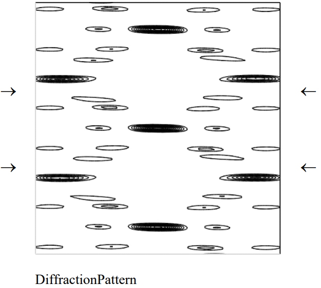
Clearly the naive model diffraction pattern presented here captures several important features of the experimental diffraction pattern. Among those are the characteristic X-shaped cross of the diffraction pattern and the missing fourth horizontal layer (indicated by arrows).

Lucas, Lisensky, and co-workers (4, 5) have simulated the DNA diffraction pattern using the optical transform method. This tutorial might therefore be considered to be a theoretical companion to their more empirical approach to the subject.

References:

1. Watson, J. D.; Crick, F. H. C. Nature 1953, 171, 737.
2. Franklin, R. E.; Gosling, R. G. Nature 1953, 171, 740.
3. Cochran, W.; Crick, F. H. C.; Vand, V. Acta Crystallogr. 1952, 5, 581.
4. Lucas, A. A.; Lambin, Ph.; Mairesse, R.; Mathot, M. J. Chem. Educ. 1999, 76, 378.
5. Lisensky, G. C.; Lucas, A. A.; Nordell, K. J.; Jackelen, A. L.; Condren, S. M.; Tobe, R. H.; Ellis, A. B. DNA Optical Transform Kit; Institute for Chemical Education: University of Wisconsin, WI, 1999.

A brief discussion of the impact of rotational symmetry in determining diffraction patterns and the concept of the quasi-crystal can be found at the following tutorial.

Crystal Structure, Rotational Symmetry and Quasicrystals

Prior to 1991 crystals were defined to be solids having only 2-, 3-, 4- and 6-fold rotational symmetry because only these rotational symmetries have the required translational periodicity to build the long-range order of a crystalline solid. Long-range order is synonymous with periodicity, requiring some unit structure which repeats itself by translation in all directions infinitely. It is easy to demonstrate that a pentagon, with 5-fold rotational symmetry cannot be used as a unit cell to create long-range order in a plane or in three-dimensions.

The justification for this definition was that solid structures with 2-, 3-, 4- and 6-fold rotational symmetry yield discrete diffraction patterns that also have translational periodicity. Another way to put this is to say that solid structures with 2-, 3-, 4- and 6-fold rotational symmetry have reciprocal lattices that also have translational periodicity. Yet, another way to put this, of course, is that the Fourier transforms of geometries with 2-, 3-, 4- and 6-fold rotational symmetry yield lattice-like momentum distributions with translational periodicity. This latter statement is preferred by the author because it emphasizes that diffraction patterns are actually the momentum distributions of the diffracted particles.

The key in this latter interpretation is that diffraction experiments involve an initial spatial localization of the radiation through interaction with the crystal lattice, followed as required by the uncertainty principle, a delocalization of the momentum distribution in the detection plane.

Let’s look at some examples. First we examine the Fourier transforms of two mini-lattices with two- and three-fold rotational symmetry.

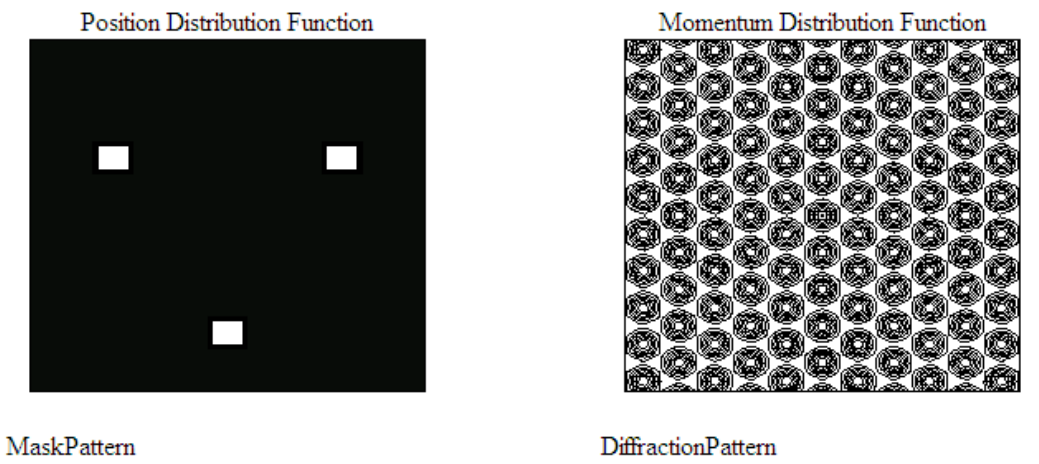
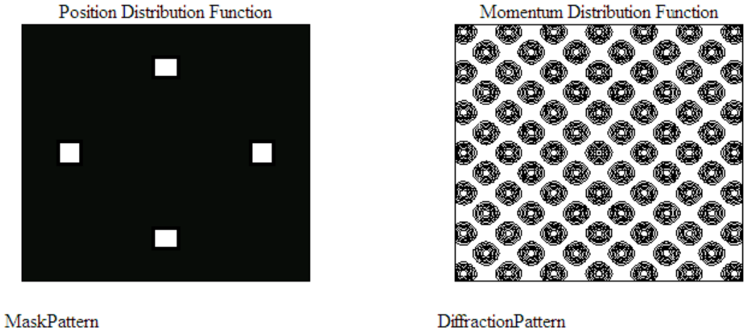
Clearly both diffraction patterns exhibit translational periodicity, their repeating units being a 90 degree rotation of the spatial structure. Next we look at four-fold rotational symmetry and see that the unit cell is obvious.

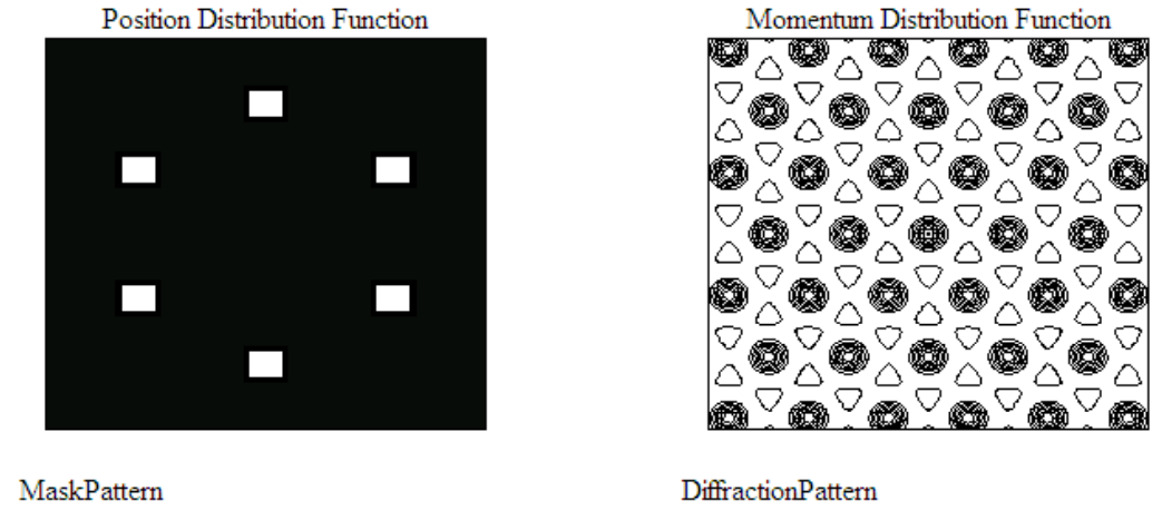
Six-fold rotational symmetry is more interesting than the previous three examples, but again the unit cell is easy to find.

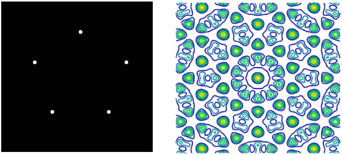
Now look at what happens when we consider 5-fold symmetry – the diffraction pattern generated by a pentagon.

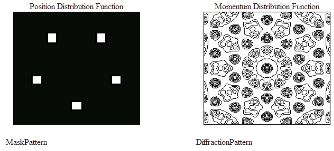
The unit cell, the universal repeating unit, is gone. The diffraction pattern is well-defined, it has rotational symmetry and it is appealing, but it does not satisfy the criterion for translational periodicity. That’s why 5-fold rotational symmetry is excluded from the list of symmetries that can generate diffraction patterns that have translational periodicity, and why by definition crystalline solids are not supposed to have 5-fold axes, or rotational axes greater than order six.

However, in 1984 an international research team consisting of D. Shechtman, I. Blech, D. Gratias and J. W. Cahn, published “Metallic phase with long-range orientational order and no translational symmetry” in Physical Review Letters 53, 1951-1953 (1984). The crystalline metallic phases they studied produced discrete diffraction patterns that were characteristic of the 5- and 10-fold rotational symmetry axes that were prohibited by the accepted definition of a crystalline solid.

In the face of this contradictory evidence, 5-fold rotational symmetry and a well-defined diffraction pattern, the International Union of Crystallography in 1991 redefined crystal to mean any solid having a discrete diffraction pattern. However, the solid phases discovered by Shechtman and his co-workers go by the name quasicrystals, indicating that they don’t quite have the same stature as those that don’t violate the rotational symmetry rule.

The striking diffraction pattern created by a pentagon of point scatterers is shown below.

In these recent examples we have been Fourier transforming from coordinate space to momentum space because the momentum distribution function is the diffraction pattern, and our experiments are set up in coordinate space. In quantum mechanics an experiment requires two steps: state preparation followed by a measurement. State preparation occurs at the slit screen and measurement at the detection screen. The following link shows how to go from the coordinate representation to the momentum representation and back again.

Single Slit Diffraction and the Fourier Transform

Slit width: \(w : = 1\)

Coordinate‐space wave function: \(\Psi(\mathrm{x}, \mathrm{w}) :=\text { if }\left[\left(\mathrm{x} \geq-\frac{\mathrm{w}}{2}\right) \cdot\left(\mathrm{x} \leq \frac{\mathrm{w}}{2}\right), 1,0\right]\)

\[
x :=\frac{-w}{2}, \frac{-w}{2}+0.005 \dots \frac{w}{2}
\nonumber \]

A Fourier transform of the coordinate‐space wave function yields the momentum wave function and the momentum distribution function, which is the diffraction pattern.

\[
\Phi\left(\mathrm{p}_{\mathrm{x}}, \mathrm{w}\right) :=\frac{1}{\sqrt{2 \cdot \pi \cdot \mathrm{w}}} \cdot \int_{-\frac{\mathrm{w}}{2}}^{\frac{\mathrm{w}}{2}} \exp \left(-\mathrm{i} \cdot \mathrm{p}_{\mathrm{x}} \cdot \mathrm{x}\right) d x \text { simplify } \rightarrow \frac{\sqrt{2} \cdot \sin \left(\frac{\mathrm{p}_{\mathrm{x}} \cdot \mathrm{w}}{2}\right)}{\sqrt{\pi} \cdot \mathrm{p}_{\mathrm{x}} \cdot \sqrt{\mathrm{w}}}
\nonumber \]

Now Fourier transform the momentum wave function back to coordinate space and display result. This is done numerically using large limits of integration for momentum.

\[
\Psi(x, w) :=\int_{-5000}^{5000} \frac{\frac{1}{2} \sin \left(\frac{1}{2} \cdot w \cdot p_{x}\right)}{\pi^{\frac{1}{2}} \cdot w^{\frac{1}{2}} \cdot p_{x}} \cdot \frac{\exp \left(i \cdot p_{x} \cdot x\right)}{\sqrt{2 \cdot \pi}} d p_{x}
\nonumber \]