1.79: The Harmonic Oscillator and the Uncertainty Principle

In atomic units the wave function in coordinate space for an harmonic oscillator with reduced mass, \(\mu\), equal to one and force constant k is given by,

\[
\Psi(\mathrm{x}, \mathrm{k}, \mu) :=\left(\frac{\sqrt{\mathrm{k} \cdot \mu}}{\pi}\right)^{\frac{1}{4}} \cdot \exp \left(-\sqrt{\mathrm{k} \cdot \mu \cdot} \frac{\mathrm{x}^{2}}{2}\right)
\nonumber \]

This function is easily Fourier transformed into momentum space:

\[
\Phi(\mathrm{p}, \mathrm{k}, \mu) :=\frac{1}{\sqrt{2 \cdot \pi}} \cdot \int_{-\infty}^{\infty} \exp (-\mathrm{i} \cdot \mathrm{p} \cdot \mathrm{x}) \cdot \Psi(\mathrm{x}, \mathrm{k}, \mu) \mathrm{dx} \Bigg| \begin{array}{l}{\text { assume, } \mathrm{k}>0} \\ {\text { assume, } \mu>0} \rightarrow \frac{e^{-\frac{p^{2}}{2 \cdot \sqrt{\mu} \cdot \sqrt{k}}}}{\pi^{\frac{1}{4}} \cdot \mu^{\frac{1}{8}} \cdot k^{\frac{1}{8}}}\\ {\text { simplify }}\end{array}
\nonumber \]

The force constant for \(\mu\)=1 controls the probability distribution in coordinate ((\Psi\)(x)²) and momentum (\(\Phi\)(p)²) space. For k = 1 the coordinate and momentum distributions are identical as is shown below.

For larger values of k the coordinate-space distribution decreases in breadth while the momentum distribution increases. For values of k less than 1, the reverse occurs; the coordinate-space distribution increases in breadth while the momentum distribution becomes narrower.

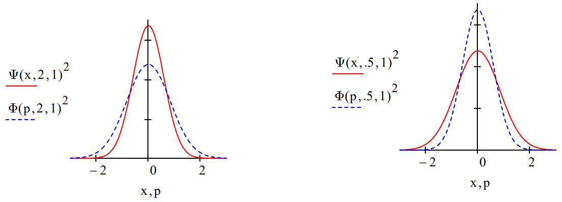
This is an illustration of the Uncertainty Principle: the more sharply defined position is, the greater the uncertainty in momentum. Conversely, the greater the uncertainty in position, the more sharply the momentum is defined.

Tunneling occurs in the simple harmonic oscillator. The classical turning point is that position at which the total energy is equal to the potential energy. In other words kinetic energy is zero and the oscillators direction is going to reverse. For the ground state the classical turning point is,

\[
\mathrm{E}=\frac{1}{2} \cdot \sqrt{\frac{\mathrm{k}}{\mu}}=\frac{\mathrm{p}^{2}}{2 \cdot \mu}+\frac{1}{2} \cdot \mathrm{k} \cdot \mathrm{x}^{2}
\nonumber \]

\[
\frac{1}{2} \cdot \sqrt{\frac{\mathrm{k}}{\mu}}=\frac{1}{2} \cdot \mathrm{k} \cdot \mathrm{x}^{2} \text { solve, }, \mathrm{x} \rightarrow \left[\begin{array}{c}{\frac{\left(\frac{k}{\mu}\right)^{\frac{1}{4}}}{\sqrt{k}}} \\ {-\frac{\left(\frac{k}{\mu}\right)^{\frac{1}{4}}}{\sqrt{k}}}\end{array}\right]
\nonumber \]

The probability that tunneling occurs is independent of the values of k and \(\mu\).

\[
2 \cdot\left[\int_{\frac{1}{(k \cdot \mu)^{\frac{1}{4}}}}^{\infty} \Psi(x, k, \mu)^{2} d x\right] \Bigg| \begin{array}{l}{\text { assume, } \mathrm{k}>0} \\ {\text { assume, } \mu>0 \rightarrow 1-\operatorname{erf}(1)=0.157} \\ {\text { simplify }}\end{array}
\nonumber \]

It is also possible to calculate the tunneling probability using the momentum wave function. Classically the maximum magnitude of momentum is achieved when the potential energy is zero, so that the total energy is equal to the kinetic energy.

\[
\frac{1}{2} \cdot \sqrt{\frac{\mathrm{k}}{\mu}}=\frac{\mathrm{p}^{2}}{2 \cdot \mu} \text { solve, } \mathrm{p} \rightarrow \left[\begin{array}{c}{\sqrt{\mu} \cdot\left(\frac{\mathrm{k}}{\mu}\right)^{\frac{1}{4}}} \\ {-\sqrt{\mu} \cdot\left(\frac{\mathrm{k}}{\mu}\right)^{\frac{1}{4}}}\end{array}\right]
\nonumber \]

Thus momentum can have values in the range shown above, depending on the magnitude of the potential energy. Values outside this range are classically forbidden. Therefore the tunneling probability in momentum space is,

\[
2 \cdot \int_{(\mathrm{k} \cdot \mu)^{\frac{1}{4}}}^{\infty} \Phi(\mathrm{p}, \mathrm{k}, \mu)^{2} \mathrm{dp} \Bigg| \begin{array}{l}{\text { assume, } \mathrm{k}>0} \\ {\text { assume, } \mu>0 \rightarrow 1-\operatorname{erf}(1)=0.157} \\ {\text { simplify }}\end{array}
\nonumber \]

It is not surprising that the momentum and coordinate calculations agree.