
1.62: Examining the Wigner Distribution Using Dirac Notation
- Page ID
- 156417

Expressing the Wigner distribution function in Dirac notation reveals its resemblance to a classical trajectory in phase space.
References to the Wigner distribution function [1-3] and the phase-space formulation of quantum mechanics are becoming more frequent in the pedagogical and review literature [4-26]. There have also been several important applications reported in the recent research literature [27, 28]. Other applications of the Wigner distribution are cited in Ref. 25.
The purpose of this note is to demonstrate that when expressed in Dirac notation the Wigner distribution resembles a classical phase-space trajectory. The Wigner distribution can be generated from either the coordinate- or momentum-space wave function. The coordinate-space wave function will be employed here and the Wigner transform using it is given in equation (1) for a one-dimensional example in atomic units.
\[
W(p, x)=\frac{1}{2 \pi} \int_{-\infty}^{\infty} \Psi^{*}\left(x+\frac{s}{2}\right) \Psi\left(x-\frac{s}{2}\right) e^{i p s} d s \tag{1}
\nonumber \]
In Dirac notation the first two terms of the integrand are written as follows,
\[
\Psi^{*}\left(x+\frac{s}{2}\right)=\left\langle\Psi | x+\frac{s}{2}\right\rangle \qquad \Psi\left(x-\frac{s}{2}\right)=\left\langle x-\frac{s}{2} | \Psi\right\rangle \tag{2}
\nonumber \]
Assigning 1/2\(\pi\) to the third term and utilizing the momentum eigenfunction in coordinate space and its complex conjugate we have,
\[
\frac{1}{2 \pi} \mathrm{e}^{i p s}=\frac{1}{\sqrt{2 \pi}} \mathrm{e}^{i p\left(x+\frac{s}{2}\right)} \frac{1}{\sqrt{2 \pi}} \mathrm{e}^{-i p\left(x-\frac{s}{2}\right)}=\left\langle x+\frac{s}{2} | p\right\rangle\left\langle p | x-\frac{s}{2}\right\rangle \tag{3}
\nonumber \]
Substituting equations (2) and (3) into equation (1) yields after arrangement
\[
W(x, p)=\int_{-\infty}^{+\infty}\left\langle\Psi | x+\frac{s}{2}\right\rangle\left\langle x+\frac{s}{2} | p\right\rangle\left\langle p | x-\frac{s}{2}\right\rangle\left\langle x-\frac{s}{2} | \Psi\right\rangle d s \tag{4}
\nonumber \]
The four Dirac brackets are read from right to left as follows: (1) is the amplitude that a particle in the state \(\Psi\) has position (x - s/2); (2) is the amplitude that a particle with position (x - s/2) has momentum p; (3) is the amplitude that a particle with momentum p has position (x + s/2); (4) is the amplitude that a particle with position (x + s/2) is (still) in the state \(\Psi\). Thus, in Dirac notation the integrand is the quantum equivalent of a classical phase-space trajectory for a quantum system in the state \(\Psi\).
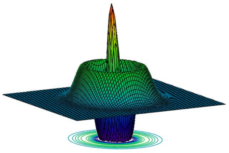
Integration over s creates a superposition of all possible quantum trajectories of the state Ψ, which interfere constructively and destructively, providing a quasi-probability distribution in phase space. As an example, the Wigner probability distribution for a double-slit experiment is shown in the figure below [14, 27]. The oscillating positive and negative values in the middle of the Wigner distribution signify the interference associated with a quantum superposition, distinguishing it from a classical phase-space probability distribution. In the words of Leibfried et al. [14], the Wigner function is a “mathematical construct for visualizing quantum trajectories in phase space.”

Wigner distribution function for the double-slit experiment.
The Wigner double- and triple-slit distribution functions are calculated in the following tutorials.
Wigner Distribution for the Double Slit Experiment
Wigner Distribution for the Triple Slit Experiment
Examples of the generation and use of the Wigner distribution are available in the following tutorials.
Wigner Distribution for the Particle in a Box
Quantum Calculations on the Hydrogen Atom in Coordinate, Momentum and Phase Space
Variation Method Using the Wigner Function: The Feshbach Potential
The Wigner Distribution Function for the Harmonic Oscillator
Given the quantum number this Mathcad file calculates the Wigner distribution function for the specified harmonic oscillator eigen state.
Quantum number: \(\mathrm{n} :=2\)
Harmonic oscillator eigenstate:
\[
\Psi(x) :=\frac{1}{\sqrt{2^{n} \cdot n ! \sqrt{\pi}}} \cdot \operatorname{Her}(n, x) \cdot \exp \left(-\frac{x^{2}}{2}\right)
\nonumber \]
Calculate the Wigner distribution:
\[
\mathrm{W}(\mathrm{x}, \mathrm{p}) :=\frac{1}{\pi^{\frac{3}{2}}} \cdot \int_{-\infty}^{\infty} \Psi\left(\mathrm{x}+\frac{\mathrm{s}}{2}\right) \cdot \exp (\mathrm{i} \cdot \mathrm{s} \cdot \mathrm{p}) \cdot \Psi\left(\mathrm{x}-\frac{\mathrm{s}}{2}\right) \mathrm{ds}
\nonumber \]
Display the Wigner distribution:
\[
\mathrm{N} :=80 \qquad \mathrm{i} :=0 \ldots \mathrm{N} \qquad x_{i} :=-4+\frac{8 \cdot i}{N} \\ \mathrm{j} :=0 \ldots \mathrm{N} \qquad \mathrm{p}_{\mathrm{j}} :=-5+\frac{10 \cdot \mathrm{j}}{\mathrm{N}} \qquad \text{Wigner}_{i, j}:=W\left(x_{i}, p_{j}\right)
\nonumber \]
Wigner, Wigner
Phase-space quantum mechanical calculations using the Wigner distribution are compared with coordinate- and momentum-space calculations in the following tutorial.
The Cliff Notes version of the above can be accessed in the following tutorial.
Literature cited:
[1] E. P. Wigner, “On the quantum correction for thermodynamic equilibrium,” Phys. Rev. 40, 749 – 759 (1932).
[2] M. Hillery, R. F. O’Connell, M. O. Scully, and E. P. Wigner, “Distribution functions in physics: Fundamentals,” Phys. Rep. 106, 121 – 167 (1984).
[3] Y. S. Kim and E. P. Wigner, “Canonical transformations in quantum mechanics,” Am. J. Phys. 58, 439 – 448 (1990).
[4] J. Snygg, “Wave functions rotated in phase space,” Am. J. Phys. 45, 58 – 60 (1977).
[5] N. Mukunda, “Wigner distribution for angle coordinates in quantum mechanics,” Am. J. Phys. 47, 192 – 187 (1979).
[6] S. Stenholm, “The Wigner function: I. The physical interpretation,” Eur. J. Phys. 1, 244 – 248 (1980).
[7] G. Mourgues, J. C. Andrieux, and M. R. Feix, “Solutions of the Schrödinger equation for a system excited by a time Dirac pulse of pulse of potential. An example of the connection with the classical limit through a particular smoothing of the Wigner function,” Eur. J. Phys. 5, 112 – 118 (1984).
[8] M. Casas, H. Krivine, and J. Martorell, “On the Wigner transforms of some simple systems and their semiclassical interpretations,” Eur. J. Phys. 12, 105 – 111 (1991).
[9] R. A. Campos, “Correlation coefficient for incompatible observables of the quantum mechanical harmonic oscillator,” Am. J. Phys. 66, 712 – 718 (1998).
[10] H-W Lee, “Spreading of a free wave packet,” Am. J. Phys. 50, 438 – 440 (1982).
[11] D. Home and S. Sengupta, “Classical limit of quantum mechanics,” Am. J. Phys. 51, 265 – 267 (1983).
[12] W. H. Zurek, “Decoherence and the transition from quantum to classical,” Phys. Today 44, 36 – 44 (October 1991).
[13] M. C. Teich and B. E. A. Saleh, “Squeezed and antibunched light,” Phys. Today 43, 26 – 34 (June 1990).
[14] D. Leibfried, T. Pfau, and C. Monroe, “Shadows and mirrors: Reconstructing quantum states of motion,” Phys. Today 51, 22 – 28 (April 1998).
[15] W. P. Schleich and G. Süssmann, “A jump shot at the Wigner distribution,” Phys. Today 44, 146 – 147 (October 1991).
[16] R. A. Campos, “Correlation coefficient for incompatible observables of the quantum harmonic oscillator,” Am. J. Phys. 66, 712 – 718 (1998).
[17] R. A. Campos, “Wigner quasiprobability distribution for quantum superpositions of coherent states, a Comment on ‘Correlation coefficient for incompatible observables of the quantum harmonic oscillator,’” Am. J. Phys. 67, 641 – 642 (1999).
[18] C. C. Gerry and P. L. Knight, “Quantum superpositions and Schrödinger cat states in quantum optics,” Am. J. Phys. 65, 964 – 974 (1997).
[19] K. Ekert and P. L. Knight, “Correlations and squeezing of two-mode oscillations,” Am. J. Phys. 57, 692 – 697 (1989).
[20] P. J. Price, “Quantum hydrodynamics and virial theorems,” Am. J. Phys. 64, 446 – 448 (1995).
[21] M. G. Raymer, “Measuring the quantum mechanical wave function,” Contemp. Phys. 38, 343 – 355 (1997).
[22] H-W Lee, A. Zysnarski, and P. Kerr, “One-dimensional scattering by a locally periodic potential,” Am. J. Phys. 57, 729 – 734 (1989).
[23] A. Royer, “Why are the energy levels of the quantum harmonic oscillator equally spaced?” Am. J. Phys. 64, 1393 – 1399 (1996).
[24] D. F. Styer, et al., “Nine formulations of quantum mechanics,” Am. J. Phys. 70, 288 – 297 (2002).
[25] M. Belloni, M. A. Doncheski, and R. W. Robinett, “Wigner quasi-probability distribution for the infinite square well: Energy eigenstates and time-dependent wave packets,” Am. J. Phys. 72, 1183 – 1192 (2004).
[26] W. B. Case, “Wigner functions and Weyl transforms for pedestrians,” Am. J. Phys. 76, 937 – 946 (2008).
[27] Ch. Kurtsiefer, T. Pfau, and J. Mlynek, “Measurement of the Wigner function of an ensemble of helium atoms,” Nature 386, 150 – 153 (1997).
[28] W. H. Zurek, “Sub-Planck structure in phase space and its relevance for quantum decoherence,” Nature 412, 712 – 717 (2001).