1.44: Which Path Information and the Quantum Eraser

This tutorial examines the real reason which‐way information destroys the double‐slit diffraction pattern and how the so‐called ʺquantum eraserʺ restores it. The traditional double‐slit experiment is presented schematically below.

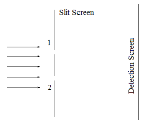
The wave function for a photon illuminating the slit screen is written as a superposition of the photon being present at both slits simultaneously.

\[
| \Psi \rangle=\frac{1}{\sqrt{2}}\left[ | x_{1}\right\rangle+| x_{2} \rangle ]
\nonumber \]

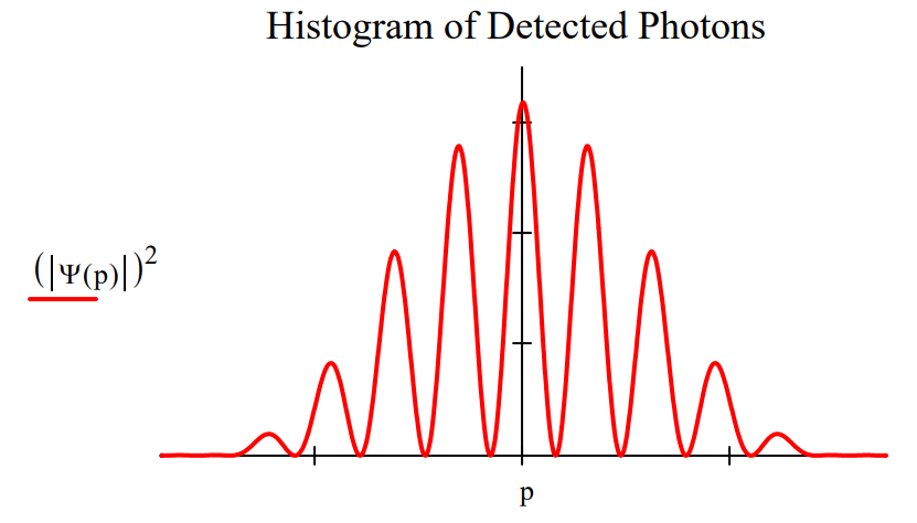
The diffraction pattern is calculated by projecting this superposition into momentum space. This is a Fourier transform for which the mathematical details can be found in the Appendix.

\[
\Psi(p)=\langle p | \Psi\rangle=\frac{1}{\sqrt{2}}\left[\left\langle p | x_{1}\right\rangle+\left\langle p | x_{2}\right\rangle\right]
\nonumber \]

The well‐known double‐slit diffraction pattern is displayed below.

When polarization markers are attached to the slits we have the following schematic of the double‐slit experiment with so‐called which‐way information.

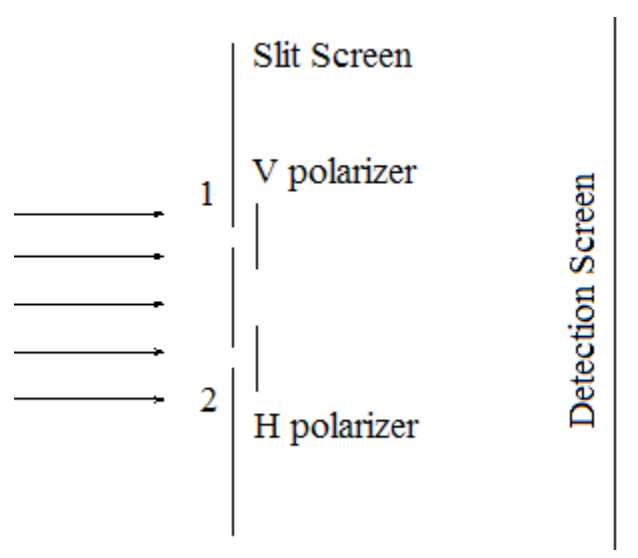
According to the Encyclopedia Britannica, Fresnel and Arago ʺusing an apparatus based on Youngʹs [double‐slit] experimentʺ observed that ʺtwo beams polarized in mutually perpendicular planes never yield fringes.ʺ We now look at the quantum mechanical explanation of this phenomena. Fresnel and Arago, working during the 19th Century, provided a valid classical explanation.

The coordinate and momentum wave functions now become,

\[
| \Psi^{\prime} \rangle=\frac{1}{\sqrt{2}}\left[ | x_{1}\right\rangle | V \rangle+| x_{2} \rangle | H \rangle ] \quad \text { where } \quad | \mathrm{V} \rangle=\left( \begin{array}{l}{1} \\ {0}\end{array}\right) \quad | \mathrm{H} \rangle=\left( \begin{array}{l}{0} \\ {1}\end{array}\right)
\nonumber \]

\[
\Psi^{\prime}(p)=\left\langle p | \Psi^{\prime}\right\rangle=\frac{1}{\sqrt{2}}\left[\left\langle p | x_{1}\right\rangle | V\right\rangle+\left\langle p | x_{2}\right\rangle | H \rangle ]
\nonumber \]

This leads to the following momentum distribution at the detection screen. The highly visible interference fringes have disappeared leaving a single‐slit diffraction pattern, but the areas of the two histograms are the same. This is demonstrated later.

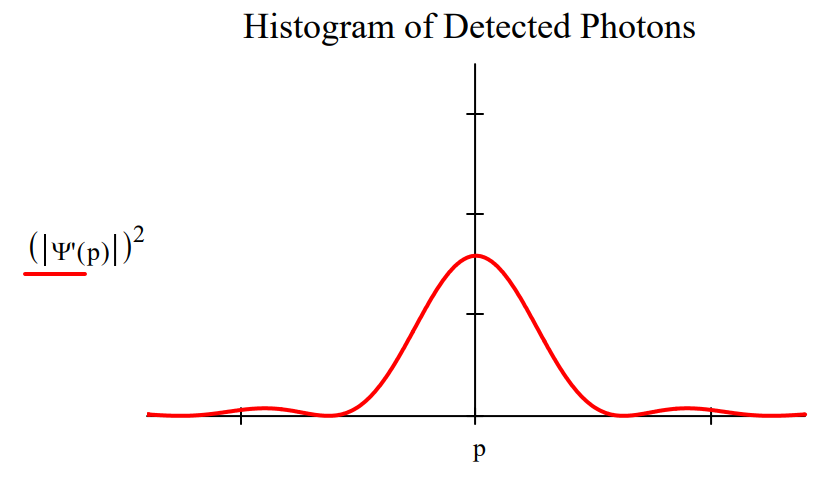
The usual explanation for this effect is that it is now possible to know which slit the photons went through, and that such knowledge destroys the interference fringes because the photons are no longer in a superposition of passing through both slits, but rather a mixture of passing through one slit or the other.

However, a more reasonable explanation is that the tags are orthogonal polarization states, and because of this the interference (cross) terms in the momentum distribution, \(\left|\Psi^{\prime}(\mathrm{p})\right|^{2}\), vanish leaving a pattern at the detection screen which is the sum of two single‐slit diffraction patterns, one from the upper slit and the other from the lower slit.

That this is a reasonable analysis is confirmed when the so‐called quantum eraser, a diagonal polarizer, is placed before the detection screen as diagramed below.

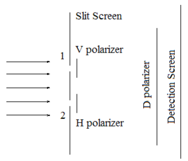
Projection of \(\Psi^{'}\) (p) onto \(\langle D | \) accounts for the action of the diagonal polarizer, yielding the following wave function after the diagonal polarizer.

\[
| \Psi^{\prime \prime} \rangle=\left\langle D | \Psi^{\prime}\right\rangle=\frac{1}{\sqrt{2}}\left[ | x_{1}\right\rangle\langle D | V\rangle+| x_{2} \rangle\langle D | H\rangle ]=\frac{1}{2}\left[ | x_{1}\right\rangle+| x_{2} \rangle ] \quad \text{where} \quad | D \rangle=\frac{1}{\sqrt{2}} \left( \begin{array}{l}{1} \\ {1}\end{array}\right)
\nonumber \]

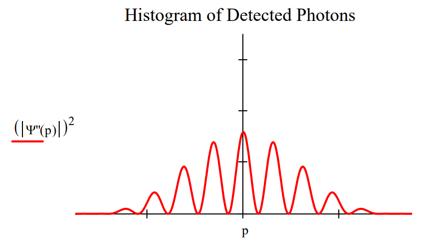
The Fourier transform of \(| \Psi^{\prime \prime}\rangle\) yields the momentum wave function and ultimately the momentum distribution function which is the diffraction pattern.

\[
\Psi^{\prime \prime}(p)=\left\langle p | \Psi^{''}\right\rangle=\frac{1}{2}\left[\left\langle p | x_{1}\right\rangle+\left\langle p | x_{2}\right\rangle\right]
\nonumber \]

The diagonal polarizer is called a quantum eraser because it appears to erase the which‐path information provided by the H/V polarizers. However, it is clear from this analysis that the diagonal polarizer doesnʹt actually erase, it passes the diagonal component of \(| \Psi^{\prime \prime}\rangle\) which then shows an attenuated (by half) version of the original diffraction pattern produced by \(| \Psi\rangle\). If which‐path erasure was occurring the integral on the right would equal 1.0.

\[
\int_{-\infty}^{\infty}(|\Psi(\mathrm{p})|)^{2} \mathrm{dp} \text { float }, 2 \rightarrow 1.0
\nonumber \]

\[
\int_{-\infty}^{\infty}\left(|\Psi^{\prime \prime}(\mathrm{p})|\right)^{2} \mathrm{d} p \text { float }, 2 \rightarrow 1.0
\nonumber \]

\[
\int_{-\infty}^{\infty}\left(|\Psi^{\prime \prime}(\mathrm{p})|\right)^{2} \mathrm{dp} \text { float }, 2 \rightarrow 0.50
\nonumber \]

Appendix

For infinitesimally thin slits the momentum‐space wave function is,

\[
\Psi(p)=\langle p | \Psi\rangle=\frac{1}{\sqrt{2}}\left[\left\langle p | x_{1}\right\rangle+\left\langle p | x_{2}\right\rangle\right]=\frac{1}{\sqrt{2}}\left[\frac{1}{\sqrt{2 \pi}} \exp \left(-i p x_{1}\right)+\frac{1}{\sqrt{2 \pi}} \exp \left(-i p x_{2}\right)\right]
\nonumber \]

Assuming a slit width \(\delta\) the calculations of \(\Psi\)(p), \(\Psi^{ʹ}\)(p) and \(\Psi^{ʹʹ}\)(p) are carried out as follows:

Position of first slit: \(\mathbf{x}_{1} \equiv 0\)

Position of second slit: \(\mathrm{x}_{2} \equiv 1\)

Slit width: \(\delta \equiv 0.2\)

\[
\Psi(p) \equiv \frac{\int_{x_{1}-\frac{\delta}{2}}^{x_{1}+\frac{\delta}{2}} \frac{1}{\sqrt{2 \cdot \pi}} \cdot \exp (-i \cdot p \cdot x) \cdot \frac{1}{\sqrt{\delta}} d x+\int_{x_{2}-\frac{\delta}{2}}^{x_{2}+\frac{\delta}{2}} \frac{1}{\sqrt{2 \cdot \pi}} \cdot \exp (-i \cdot p \cdot x) \cdot \frac{1}{\sqrt{\delta}} d x}{\sqrt{2}}
\nonumber \]

\[
\Psi^{'}(p)\equiv \frac{\int_{x_{1}-\frac{\delta}{2}}^{x_{1}+\frac{\delta}{2}} \frac{1}{\sqrt{2 \cdot \pi}} \cdot \exp (-i \cdot p \cdot x) \cdot \frac{1}{\sqrt{\delta}} d x \cdot \begin{pmatrix} 1 \\ 0 \end{pmatrix} +\int_{x_{2}-\frac{\delta}{2}}^{x_{2}+\frac{\delta}{2}} \frac{1}{\sqrt{2 \cdot \pi}} \cdot \exp (-i \cdot p \cdot x) \cdot \frac{1}{\sqrt{\delta}} d x \cdot \begin{pmatrix} 0 \\ 1 \end{pmatrix}}{\sqrt{2}}
\nonumber \]

\[
\Psi^{'}(p)\equiv \frac{\frac{1}{\sqrt{2}} \cdot \begin{pmatrix} 1 \\ 1 \end{pmatrix}^{T} \cdot \left[ \int_{x_{1}-\frac{\delta}{2}}^{x_{1}+\frac{\delta}{2}} \frac{1}{\sqrt{2 \cdot \pi}} \cdot \exp (-i \cdot p \cdot x) \cdot \frac{1}{\sqrt{\delta}} d x \cdot \begin{pmatrix} 1 \\ 0 \end{pmatrix} +\int_{x_{2}-\frac{\delta}{2}}^{x_{2}+\frac{\delta}{2}} \frac{1}{\sqrt{2 \cdot \pi}} \cdot \exp (-i \cdot p \cdot x) \cdot \frac{1}{\sqrt{\delta}} d x \cdot \begin{pmatrix} 0 \\ 1 \end{pmatrix} \right]}{\sqrt{2}}
\nonumber \]