1.42: The Quantum Eraser

Paul Kwiat and an undergraduate research assistant published ʺA Do‐It‐Yourself Quantum Eraserʺ in the May 2007 issue of Scientific American. The purpose of this tutorial is to show the quantum math behind the laser demonstrations illustrated in this article.

The quantum mechanics behind the quantum eraser is very similar to that previously used to analyze the double‐slit experiment with polarized light. By way of review we recall that the interference pattern produced in the traditional double‐slit experiment is actually the momentum distribution created by the double‐slit geometry. In other words, the interference pattern is the Fourier transform of the spatial geometry of the slits.

\[
| \Psi \rangle=\frac{1}{\sqrt{2}}\left[ | x_{1}\right\rangle+| x_{2} \rangle ]
\nonumber \]

\[
\langle p | \Psi\rangle=\frac{1}{\sqrt{2}}\left[\left\langle p | x_{i}\right\rangle+\left\langle p | x_{2}\right\rangle\right]=\frac{1}{\sqrt{2}}\left[\frac{1}{\sqrt{2 \pi}} \exp \left(-i p x_{1}\right)+\frac{1}{\sqrt{2 \pi}} \exp \left(-i p x_{2}\right)\right]
\nonumber \]

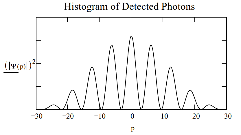
For slits of width \(\delta\) positioned as indicated below we have,

Position of first slit: \(x_{1} :=0\)

Position of second slit: \(\mathrm{x}_{2} :=1\)

Slit width: \(\delta :=0.2\)

\[\Psi (p):= \frac{\int_{\mathrm{x}_{1}-\frac{\delta}{2}}^{\mathrm{x}_{1}+\frac{\delta}{2}} \frac{1}{\sqrt{2 \cdot \pi}} \cdot \exp (-\mathrm{i} \cdot \mathrm{p} \cdot \mathrm{x}) \cdot \frac{1}{\sqrt{\delta}} \mathrm{dx}+\int_{x_{2}-\frac{\delta}{2}}^{x_{2}+\frac{\delta}{2}} \frac{1}{\sqrt{2 \cdot \pi}} \cdot \exp (-\mathrm{i} \cdot \mathrm{p} \cdot \mathrm{x}) \cdot \frac{1}{\sqrt{\delta}} d x}{\sqrt{2}} \nonumber \]

yielding the following diffraction pattern.

To gain ʺwhich‐wayʺ information a vertical polarizer is placed behind the first slit and a horizontal polarizer behind the second slit. Essentially two state preparation measurements have been made yielding the following entangled superposition state. (Path and polarization information have been entangled; the path part and polarizaton part cannot be factored into a product of terms.)

\[
| \Psi \rangle=\frac{1}{\sqrt{2}}\left[ | x_{1}\right\rangle | \mathrm{V} \rangle+| x_{2} \rangle | H \rangle ]
\nonumber \]

Next come the measurements ‐ polarization state, followed by momentum distribution (the spatial distribution of photon arrivals at the detection screen). The state preparation and measurement apparatus is shown skematically below.

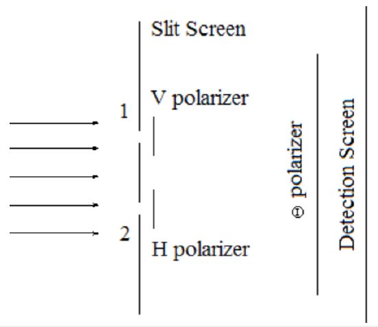
To calculate the results of these sequential measurements \(| \Psi>\) is projected onto \(<\theta, \mathrm{p} |\), yielding for slits of width \(\delta\) the following measurement state.

\[\Psi(p, \theta):=\frac{\int_{x_{1}-\frac{\delta}{2}}^{x_{1}+\frac{\delta}{2}} \frac{1}{\sqrt{2 \cdot \pi}} \cdot \exp (-\mathrm{i} \cdot \mathrm{p} \cdot \mathrm{x}) \cdot \frac{1}{\sqrt{\delta}} d x \cdot \cos (\theta)+\int_{\mathrm{x}_{2} \frac{\delta}{2}}^{\mathrm{x}_{2}+\frac{\delta}{2}} \frac{1}{\sqrt{2 \cdot \pi}} \cdot \exp (-\mathrm{i} \cdot \mathrm{p} \cdot \mathrm{x}) \cdot \frac{1}{\sqrt{\delta}} \mathrm{d} x \sin (\theta)}{\sqrt{2}} \nonumber \]

Kwiat and Hillmer create a double‐slit effect by illuminating a thin wire with a narrow laser beam which is displayed on a distant screen. A brief discussion of their demonstrations in light of the mathematics presented here follows.

• Observing the double‐slit interference effect. The quantum mechanics is outlined at the beginning of this tutorial.
• Labeling the photon path with crossed polarizers (figure above without the third polarizer in front of the detection screen). The quantum math for this demonstration can be found in the previous tutorial, ʺThe Double‐Slit Experiment with Polarized Light.ʺ No interference fringes are predicted and none are observed. This effect was first observed by Fresnel and Arago in the first part of the 19th Century. It appears that this was the first example of the importance of path information in interference phenomena.
• Same as the previous demonstration, but with a third polarizer positioned in front of the detection screen. If the third polarizer is vertically (\(\theta\) = 0) or horizontally (\(\theta = \frac{\pi}{2}\)) oriented no interference fringes are observed. The first two traces in the figure below show that no fringes are predicted.
• Same as the previous demonstration, except that the third polarizer is diagonally oriented (\(\theta = \frac{\pi}{4}\)) and anti‐diagonally oriented (\(\theta = - \frac{\pi}{4}\)). Now fringes are observed and predicted, as can be seen in the third and fourth traces in the figure.

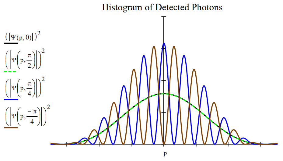
Regarding the last demonstration, the reason for the restoration of the interference fringes is that the ʺwhich‐wayʺ information provided by the crossed polarizers has been lost or erased. The vertically and horizontally polarized photons from slits 1 and 2 both have a 50% chance of passing the diagonally or anti‐diagonally oriented third polarizer. Thus, knowledge of the origin of a photon emerging from the third polarizer has been destroyed.