
6.5: s-orbitals are Spherically Symmetric
- Page ID
- 13430
The hydrogen atom wavefunctions, \(\psi (r, \theta , \varphi )\), are called atomic orbitals. An atomic orbital is a function that describes one electron in an atom. The wavefunction with \(n = 1\), \(l\) = 0 is called the 1s orbital, and an electron that is described by this function is said to be “in” the ls orbital, i.e. have a 1s orbital state. The constraints on n, \(l\), and \(m_l\) that are imposed during the solution of the hydrogen atom Schrödinger equation explain why there is a single 1s orbital, why there are three 2p orbitals, five 3d orbitals, etc. We will see when we consider multi-electron atoms, these constraints explain the features of the Periodic Table. In other words, the Periodic Table is a manifestation of the Schrödinger model and the physical constraints imposed to obtain the solutions to the Schrödinger equation for the hydrogen atom.
Visualizing the variation of an electronic wavefunction with r, \(\theta\), and \(\varphi\) is important because the absolute square of the wavefunction depicts the charge distribution (electron probability density) in an atom or molecule. The charge distribution is central to chemistry because it is related to chemical reactivity. For example, an electron deficient part of one molecule is attracted to an electron rich region of another molecule, and such interactions play a major role in chemical interactions ranging from substitution and addition reactions to protein folding and the interaction of substrates with enzymes.
We can obtain an energy and one or more wavefunctions for every value of \(n\), the principal quantum number, by solving Schrödinger's equation for the hydrogen atom. A knowledge of the wavefunctions, or probability amplitudes \(\psi_n\), allows us to calculate the probability distributions for the electron in any given quantum level. When n = 1, the wavefunction and the derived probability function are independent of direction and depend only on the distance r between the electron and the nucleus. In Figure 6.5.1 , we plot both \(\psi_1\) and \(P_1\) versus \(r\), showing the variation in these functions as the electron is moved further and further from the nucleus in any one direction. (These and all succeeding graphs are plotted in terms of the atomic unit of length, \(a_0 = 0.529 \times 10^{-8}\, cm\).)
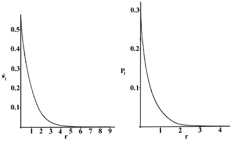
Two interpretations can again be given to the \(P_1\) curve. An experiment designed to detect the position of the electron with an uncertainty much less than the diameter of the atom itself (using light of short wavelength) will, if repeated a large number of times, result in Figure 6.5.1 for \(P_1\). That is, the electron will be detected close to the nucleus most frequently and the probability of observing it at some distance from the nucleus will decrease rapidly with increasing \(r\). The atom will be ionized in making each of these observations because the energy of the photons with a wavelength much less than 10-8 cm will be greater than \(K\), the amount of energy required to ionize the hydrogen atom. If light with a wavelength comparable to the diameter of the atom is employed in the experiment, then the electron will not be excited but our knowledge of its position will be correspondingly less precise. In these experiments, in which the electron's energy is not changed, the electron will appear to be "smeared out" and we may interpret \(P_1\) as giving the fraction of the total electronic charge to be found in every small volume element of space. (Recall that the addition of the value of Pn for every small volume element over all space adds up to unity, i.e., one electron and one electronic charge.)
Visualizing wavefunctions and charge distributions is challenging because it requires examining the behavior of a function of three variables in three-dimensional space. This visualization is made easier by considering the radial and angular parts separately, but plotting the radial and angular parts separately does not reveal the shape of an orbital very well. The shape can be revealed better in a probability density plot. To make such a three-dimensional plot, divide space up into small volume elements, calculate \(\psi ^* \psi \) at the center of each volume element, and then shade, stipple or color that volume element in proportion to the magnitude of \(\psi ^* \psi \).
We could also represent the distribution of negative charge in the hydrogen atom in the manner used previously for the electron confined to move on a plane (Figure 6.5.2 ), by displaying the charge density in a plane by means of a contour map. Imagine a plane through the atom including the nucleus. The density is calculated at every point in this plane. All points having the same value for the electron density in this plane are joined by a contour line (Figure 6.5.2 ). Since the electron density depends only on r, the distance from the nucleus, and not on the direction in space, the contours will be circular. A contour map is useful as it indicates the "shape" of the density distribution.
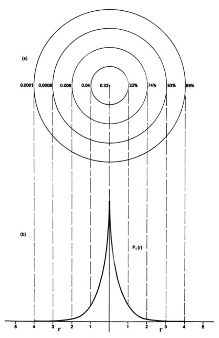
When the electron is in a definite energy level we shall refer to the \(P_n\) distributions as electron density distributions, since they describe the manner in which the total electronic charge is distributed in space. The electron density is expressed in terms of the number of electronic charges per unit volume of space, e-/V. The volume V is usually expressed in atomic units of length cubed, and one atomic unit of electron density is then e-/a03. To give an idea of the order of magnitude of an atomic density unit, 1 au of charge density e-/a03 = 6.7 electronic charges per cubic Ångstrom. That is, a cube with a length of \(0.52917 \times 10^{-8}\; cm\), if uniformly filled with an electronic charge density of 1 au, would contain 6.7 electronic charges.
For every value of the energy En, for the hydrogen atom, there is a degeneracy equal to \(n^2\). Therefore, for n = 1, there is but one atomic orbital and one electron density distribution. However, for n = 2, there are four different atomic orbitals and four different electron density distributions, all of which possess the same value for the energy, E2. Thus for all values of the principal quantum number n there are n2 different ways in which the electronic charge may be distributed in three-dimensional space and still possess the same value for the energy. For every value of the principal quantum number, one of the possible atomic orbitals is independent of direction and gives a spherical electron density distribution which can be represented by circular contours as has been exemplified above for the case of n = 1. The other atomic orbitals for a given value of n exhibit a directional dependence and predict density distributions which are not spherical but are concentrated in planes or along certain axes. The angular dependence of the atomic orbitals for the hydrogen atom and the shapes of the contours of the corresponding electron density distributions are intimately connected with the angular momentum possessed by the electron.
Methods for separately examining the radial portions of atomic orbitals provide useful information about the distribution of charge density within the orbitals. Graphs of the radial functions, \(R(r)\), for the 1s and 2s orbitals plotted in Figure 6.5.3 . The 1s function in Figure \(\PageIndex{3; left}\) starts with a high positive value at the nucleus and exponentially decays to essentially zero after 5 Bohr radii. The high value at the nucleus may be surprising, but as we shall see later, the probability of finding an electron at the nucleus is vanishingly small.
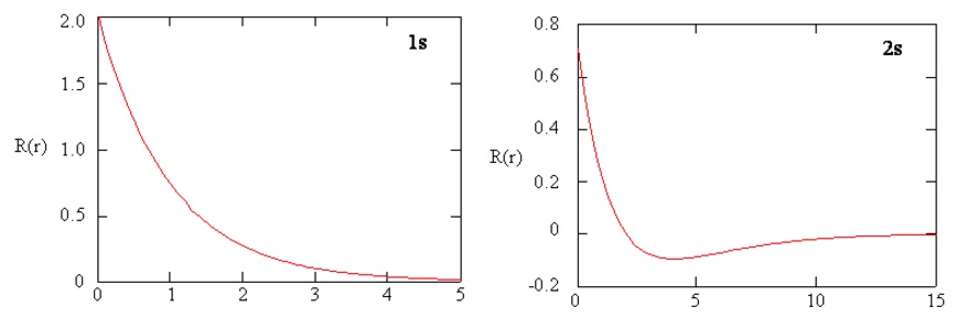
Next notice how the radial function for the 2s orbital, Figure \(\PageIndex{3; right}\), goes to zero and becomes negative. This behavior reveals the presence of a radial node in the function. A radial node occurs when the radial function equals zero other than at \(r = 0\) or \(r = ∞\). Nodes and limiting behaviors of atomic orbital functions are both useful in identifying which orbital is being described by which wavefunction. For example, all of the s functions have non-zero wavefunction values at \(r = 0\).
Examine the mathematical forms of the radial wavefunctions. What feature in the functions causes some of them to go to zero at the origin while the s functions do not go to zero at the origin?
What mathematical feature of each of the radial functions controls the number of radial nodes?
At what value of \(r\) does the 2s radial node occur?
Make a table that provides the energy, number of radial nodes, and the number of angular nodes and total number of nodes for each function with \(n = 1\), \(n=2\), and \(n=3\). Identify the relationship between the energy and the number of nodes. Identify the relationship between the number of radial nodes and the number of angular nodes.
- Answer
-
Energy
1.Particle in a Box (h2n2/8meL2)
2.Harmonic Oscillator((n+0.5)ℏω)
3.Hydrogen (-13.6eV/n2)
Number of Radial Nodes
(n-l-1)
Number of Angular Nodes
l = (n-1)
l : s =0
p = 1
d = 2
Total Number of Nodes n = 1 1. 6.02 *10-38 J/L2
2. 1.5ℏω
3. -13.6 eV
- 0 0 n = 2 1. 6.02 *10-38 J/L2
2. 2.5ℏω
3. -3.4 eV
for s: 1
for p: 0
for s: 0
for p: 1
1 n = 3 1. 6.02 *10-38 J/L2
2. 3.5ℏω
3. 1.51 eV
for s: 2
for p: 1
for d: 0
for s: 0
for p:1
for d: 2
2 For a particle in a box the energy is equivalent to \(E_n= 6.02 \times 10^{-38} n^2L^2\) where \(n\) is any value greater than and not equal to 0 and L is the length of the box.
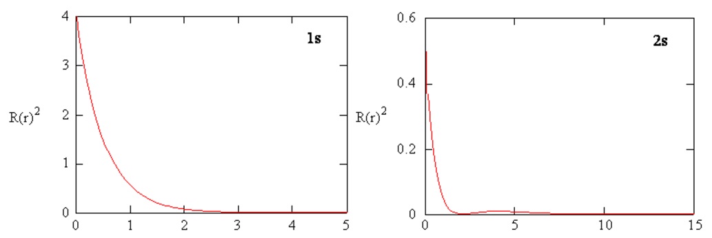
Radial probability densities for the 1s and 2s atomic orbitals are plotted in Figure 6.5.4 .
Radial Distribution Functions
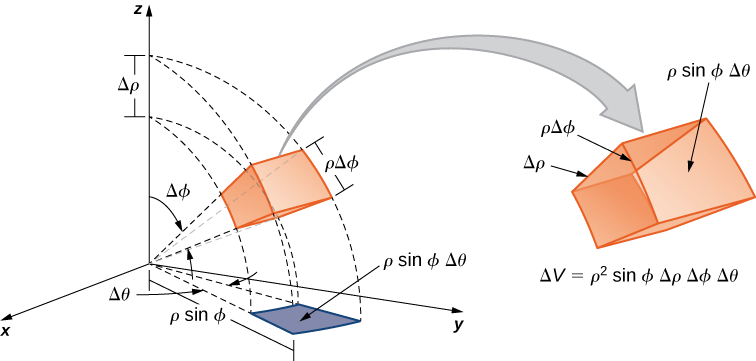
Rather than considering the amount of electronic charge in one particular small element of space, we may determine the total amount of charge lying within a thin spherical shell of space. Since the distribution is independent of direction, consider adding up all the charge density which lies within a volume of space bounded by an inner sphere of radius \(r\) and an outer concentric sphere with a radius only infinitesimally greater, say \(r + \Delta r\). The area of the inner sphere is \(4\pi r^2\) and the thickness of the shell is \(\Delta r\). Thus the volume of the shell is \(4\pi r^2 \Delta r\) and the product of this volume and the charge density P1(r), which is the charge or number of electrons per unit volume, is therefore the total amount of electronic charge lying between the spheres of radius \(r\) and \(r + \Delta r\). The product \(4\pi r^2P_n\) is given a special name, the radial distribution function.
The reader may wonder why the volume of the shell is not taken as:
\[ \dfrac{4}{3} \pi \left[ (r + \Delta r)^3 -r^3 \right] \nonumber \]
the difference in volume between two concentric spheres. When this expression for the volume is expanded, we obtain
\[\dfrac{4}{3} \pi \left(3r^2 \Delta r + 3r \Delta r^2 + \Delta r^3\right) \nonumber \]
and for very small values of \(\Delta r\) the \(3r \Delta r^2\) and \(\Delta r^3\) terms are negligible in comparison with \(3r^2\Delta r\). Thus for small values of \(\Delta r\), the two expressions for the volume of the shell approach one another in value and when \(\Delta r\) represents an infinitesimal small increment in \(r\) they are identical.
The radial distribution function is plotted in Figure 6.5.5 for the ground state of the hydrogen atom.
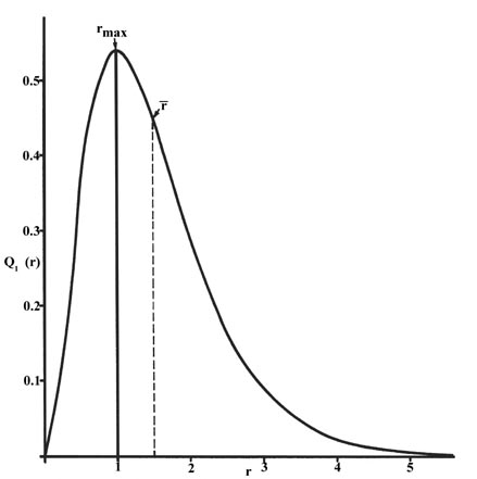
The curve passes through zero at \(r = 0\) since the surface area of a sphere of zero radius is zero. As the radius of the sphere is increased, the volume of space defined by \(4 \pi r^2Dr\) increases. However, as shown in Figure 6.5.4 , the absolute value of the electron density at a given point decreases with \(r\) and the resulting curve must pass through a maximum. This maximum occurs at \(r_{max} = a_0\). Thus more of the electronic charge is present at a distance \(a_o\), out from the nucleus than at any other value of \(r\). Since the curve is unsymmetrical, the average value of \(r\), denoted by \(\bar{r}\), is not equal to \(r_{max}\). The average value of \(r\) is indicated on the figure by a dashed line. A "picture" of the electron density distribution for the electron in the \(n = 1\) level of the hydrogen atom would be a spherical ball of charge, dense around the nucleus and becoming increasingly diffuse as the value of \(r\) is increased.
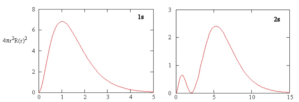
The radial distribution function gives the probability density for an electron to be found anywhere on the surface of a sphere located a distance \(r\) from the proton. Since the area of a spherical surface is \(4 \pi r^2\), the radial distribution function is given by \(4 \pi r^2 R(r) ^* R(r)\).
Radial distribution functions are shown in Figure 6.5.6 . At small values of \(r\), the radial distribution function is low because the small surface area for small radii modulates the high value of the radial probability density function near the nucleus. As we increase \(r\), the surface area associated with a given value of \(r\) increases, and the \(r^2\) term causes the radial distribution function to increase even though the radial probability density is beginning to decrease. At large values of \(r\), the exponential decay of the radial function outweighs the increase caused by the \(r^2\) term and the radial distribution function decreases.
Calculate the probability of finding a 1s hydrogen electron being found within distance \(2a_o\) from the nucleus.
- Solution
-
Note the wavefunction of hydrogen 1s orbital which is
\[ψ_{100}= \dfrac{1}{\sqrt{π}} \left(\dfrac{1}{a_0}\right)^{3/2} e^{-\rho} \nonumber \]
with \(\rho=\dfrac{r}{a_0} \).
The probability of finding the electron within \(2a_0\) distance from the nucleus will be:
\[prob= \underbrace{\int_{0}^{\pi} \sin \theta \, d\theta}_{over\, \theta} \, \overbrace{ \dfrac{1}{\pi a_0^3} \int_{0}^{2a_0} r^2 e^{-2r/a_0} dr}^{over\, r} \, \underbrace{ \int_{0}^{2\pi} d\phi }_{over\, \phi } \nonumber \]
Since \(\int_0^{\pi} \sin \theta d\theta=2\) and \( \int_0^{2\pi} d\phi=2\pi\), we have
\[ \begin{align*} prob &=2 \times 2\pi \times \dfrac{1}{\pi a_0^3} \int_0^2a_0 (-a_0/2)r^2 d e^{-2r/a_0} \\[4pt]&=\dfrac{4}{a_0^3}\left(-\dfrac{a_0}{2}\right) (r^2 e^{-2r/a_0} |_0^{2a_0} - \int_0^{2a_0} 2r e^{-2r/a_0} dr) \\[4pt]&= -\dfrac{2}{a_0^2} [(2a_0)^2 e^{-4}-0-2\int_0^{2a_0} r \left(-\dfrac{a_0}{2}\right) d e^{-2r/a_0} ] \\[4pt]&=-\dfrac{2}{a_0^2}4a_0^2 e^{-4} +\dfrac{4}{a_0^2}(-\dfrac{a_0}{2}) (r e^{-2r/a_0} |_0^{2a_0}-\int_0^{2a_0} e^{-2r/a_0} dr ) \\[4pt]&=-8e^{-4}-\dfrac{2}{a_0} \left[2a_0e^{-4}-0-(-\dfrac{a_0}{2})e^{-2r/a_0} |_0^{2a_0} \right] \\[4pt]&=-8e^{-4}-4e^{-4}-e^{2r/a_0} |_0^{2a_0} \\[4pt]&=-12 e^{-4}-(e^{-4}-1)=1-13e^{-4}=0.762 \end{align*} \nonumber \]
There is a 76.2% probability that the electrons will be within \(2a_o\) of the nucleus in the 1s eigenstate.
Summary
This completes the description of the most stable state of the hydrogen atom, the state for which \(n = 1\). Before proceeding with a discussion of the excited states of the hydrogen atom we must introduce a new term. When the energy of the electron is increased to another of the allowed values, corresponding to a new value for \(n\), \(y_n\) and \(P_n\) change as well. The wavefunctions \(y_n\) for the hydrogen atom are given a special name, atomic orbitals, because they play such an important role in all of our future discussions of the electronic structure of atoms. In general the word orbital is the name given to a wavefunction which determines the motion of a single electron. If the one-electron wavefunction is for an atomic system, it is called an atomic orbital.
Do not confuse the word orbital with the classical word and notion of an orbit. First, an orbit implies the knowledge of a definite trajectory or path for a particle through space which in itself is not possible for an electron. Secondly, an orbital, like the wavefunction, has no physical reality but is a mathematical function which when squared gives the physically measurable electron density distribution.
Contributors and Attributions
Dr. Richard F.W. Bader (Professor of Chemistry / McMaster University)
David M. Hanson, Erica Harvey, Robert Sweeney, Theresa Julia Zielinski ("Quantum States of Atoms and Molecules")