Chemistry LibreTexts

19.10: Relative Enthalpies Can Be Determined from Heat Capacity Data and Heats of Transition

  • Page ID
    13708
  • \( \newcommand{\vecs}[1]{\overset { \scriptstyle \rightharpoonup} {\mathbf{#1}} } \)

    \( \newcommand{\vecd}[1]{\overset{-\!-\!\rightharpoonup}{\vphantom{a}\smash {#1}}} \)

    \( \newcommand{\id}{\mathrm{id}}\) \( \newcommand{\Span}{\mathrm{span}}\)

    ( \newcommand{\kernel}{\mathrm{null}\,}\) \( \newcommand{\range}{\mathrm{range}\,}\)

    \( \newcommand{\RealPart}{\mathrm{Re}}\) \( \newcommand{\ImaginaryPart}{\mathrm{Im}}\)

    \( \newcommand{\Argument}{\mathrm{Arg}}\) \( \newcommand{\norm}[1]{\| #1 \|}\)

    \( \newcommand{\inner}[2]{\langle #1, #2 \rangle}\)

    \( \newcommand{\Span}{\mathrm{span}}\)

    \( \newcommand{\id}{\mathrm{id}}\)

    \( \newcommand{\Span}{\mathrm{span}}\)

    \( \newcommand{\kernel}{\mathrm{null}\,}\)

    \( \newcommand{\range}{\mathrm{range}\,}\)

    \( \newcommand{\RealPart}{\mathrm{Re}}\)

    \( \newcommand{\ImaginaryPart}{\mathrm{Im}}\)

    \( \newcommand{\Argument}{\mathrm{Arg}}\)

    \( \newcommand{\norm}[1]{\| #1 \|}\)

    \( \newcommand{\inner}[2]{\langle #1, #2 \rangle}\)

    \( \newcommand{\Span}{\mathrm{span}}\) \( \newcommand{\AA}{\unicode[.8,0]{x212B}}\)

    \( \newcommand{\vectorA}[1]{\vec{#1}}      % arrow\)

    \( \newcommand{\vectorAt}[1]{\vec{\text{#1}}}      % arrow\)

    \( \newcommand{\vectorB}[1]{\overset { \scriptstyle \rightharpoonup} {\mathbf{#1}} } \)

    \( \newcommand{\vectorC}[1]{\textbf{#1}} \)

    \( \newcommand{\vectorD}[1]{\overrightarrow{#1}} \)

    \( \newcommand{\vectorDt}[1]{\overrightarrow{\text{#1}}} \)

    \( \newcommand{\vectE}[1]{\overset{-\!-\!\rightharpoonup}{\vphantom{a}\smash{\mathbf {#1}}}} \)

    \( \newcommand{\vecs}[1]{\overset { \scriptstyle \rightharpoonup} {\mathbf{#1}} } \)

    \( \newcommand{\vecd}[1]{\overset{-\!-\!\rightharpoonup}{\vphantom{a}\smash {#1}}} \)

    \(\newcommand{\avec}{\mathbf a}\) \(\newcommand{\bvec}{\mathbf b}\) \(\newcommand{\cvec}{\mathbf c}\) \(\newcommand{\dvec}{\mathbf d}\) \(\newcommand{\dtil}{\widetilde{\mathbf d}}\) \(\newcommand{\evec}{\mathbf e}\) \(\newcommand{\fvec}{\mathbf f}\) \(\newcommand{\nvec}{\mathbf n}\) \(\newcommand{\pvec}{\mathbf p}\) \(\newcommand{\qvec}{\mathbf q}\) \(\newcommand{\svec}{\mathbf s}\) \(\newcommand{\tvec}{\mathbf t}\) \(\newcommand{\uvec}{\mathbf u}\) \(\newcommand{\vvec}{\mathbf v}\) \(\newcommand{\wvec}{\mathbf w}\) \(\newcommand{\xvec}{\mathbf x}\) \(\newcommand{\yvec}{\mathbf y}\) \(\newcommand{\zvec}{\mathbf z}\) \(\newcommand{\rvec}{\mathbf r}\) \(\newcommand{\mvec}{\mathbf m}\) \(\newcommand{\zerovec}{\mathbf 0}\) \(\newcommand{\onevec}{\mathbf 1}\) \(\newcommand{\real}{\mathbb R}\) \(\newcommand{\twovec}[2]{\left[\begin{array}{r}#1 \\ #2 \end{array}\right]}\) \(\newcommand{\ctwovec}[2]{\left[\begin{array}{c}#1 \\ #2 \end{array}\right]}\) \(\newcommand{\threevec}[3]{\left[\begin{array}{r}#1 \\ #2 \\ #3 \end{array}\right]}\) \(\newcommand{\cthreevec}[3]{\left[\begin{array}{c}#1 \\ #2 \\ #3 \end{array}\right]}\) \(\newcommand{\fourvec}[4]{\left[\begin{array}{r}#1 \\ #2 \\ #3 \\ #4 \end{array}\right]}\) \(\newcommand{\cfourvec}[4]{\left[\begin{array}{c}#1 \\ #2 \\ #3 \\ #4 \end{array}\right]}\) \(\newcommand{\fivevec}[5]{\left[\begin{array}{r}#1 \\ #2 \\ #3 \\ #4 \\ #5 \\ \end{array}\right]}\) \(\newcommand{\cfivevec}[5]{\left[\begin{array}{c}#1 \\ #2 \\ #3 \\ #4 \\ #5 \\ \end{array}\right]}\) \(\newcommand{\mattwo}[4]{\left[\begin{array}{rr}#1 \amp #2 \\ #3 \amp #4 \\ \end{array}\right]}\) \(\newcommand{\laspan}[1]{\text{Span}\{#1\}}\) \(\newcommand{\bcal}{\cal B}\) \(\newcommand{\ccal}{\cal C}\) \(\newcommand{\scal}{\cal S}\) \(\newcommand{\wcal}{\cal W}\) \(\newcommand{\ecal}{\cal E}\) \(\newcommand{\coords}[2]{\left\{#1\right\}_{#2}}\) \(\newcommand{\gray}[1]{\color{gray}{#1}}\) \(\newcommand{\lgray}[1]{\color{lightgray}{#1}}\) \(\newcommand{\rank}{\operatorname{rank}}\) \(\newcommand{\row}{\text{Row}}\) \(\newcommand{\col}{\text{Col}}\) \(\renewcommand{\row}{\text{Row}}\) \(\newcommand{\nul}{\text{Nul}}\) \(\newcommand{\var}{\text{Var}}\) \(\newcommand{\corr}{\text{corr}}\) \(\newcommand{\len}[1]{\left|#1\right|}\) \(\newcommand{\bbar}{\overline{\bvec}}\) \(\newcommand{\bhat}{\widehat{\bvec}}\) \(\newcommand{\bperp}{\bvec^\perp}\) \(\newcommand{\xhat}{\widehat{\xvec}}\) \(\newcommand{\vhat}{\widehat{\vvec}}\) \(\newcommand{\uhat}{\widehat{\uvec}}\) \(\newcommand{\what}{\widehat{\wvec}}\) \(\newcommand{\Sighat}{\widehat{\Sigma}}\) \(\newcommand{\lt}{<}\) \(\newcommand{\gt}{>}\) \(\newcommand{\amp}{&}\) \(\definecolor{fillinmathshade}{gray}{0.9}\)

    It should be stressed that there are no absolute enthalpies. All that is properly defined are differences in enthalpy ΔH and these are only defined for processes

    When dealing with enthalpies

    Define the Process

    For example for the process of:

    Process 1: heating ice from -20oC to -0oC

    We could write ΔH1 = ∫ CP,ice. dT from T=253K to T=273K = H(273) -H(253). But before moving beyond the melting point first a different process needs to take place, that of

    Process 2: melting

    This gives us ΔfusH = Hliquid - Hsolid (both at 273K!). When we heat the liquid water further to say +20oC we would have to integrate over the heat capacity of the liquid.

    Process 3: heating water from 0oC to +20oC

    We could write

    \[ΔH_3 = \int C_{P,water} dT \nonumber \]

    from T=273K to T=293K = H(293)-H(273).

    The total change in enthalpy between -20 and +20 would be the sum of the three enthalpy changes.

    \[ΔH_{total process} = ΔH_1 + Δ_{fus}H + ΔH_3 \nonumber \]

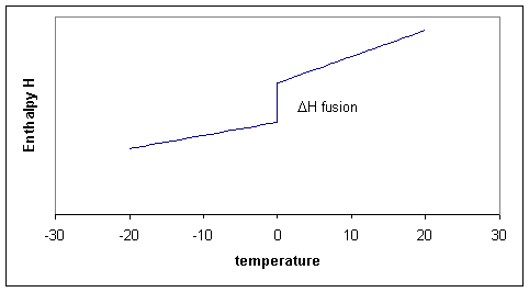
    Of course we could consider doing the same calculation for any temperature between -20 and +20 and summarize all our results in a graph. The three processes can thus schematically be shown in Figure 19.10.1 .
    alt
    Figure 19.10.1 : Schematic enthalpy function showing the jump at the melting point

    Notice that the slopes (i.e. the heat capacities!) before and after the melting point differ. The slope for the liquid is a little steeper because the liquid has more degrees of freedom and therefore the heat capacity of the liquid tends to be higher than of the solid. In the figure the enthlapy curves are shown as straight lines. This would be the case if the heat capacities are constant over the temperature interval. Although Cp is typically a 'slow' or 'weak' function of temperature it usually does change a bit, which means that the straight lines for H become curves.

    Although Cp is typically a 'slow' or 'weak' function of temperature and is well approximated as a constant.

    Notice that for process two, the temperature is constant, that means that \(ΔT\) or \(dT\) is zero, but ΔH is finite, consequently ΔH/ΔT is infinitly large. Taking the limit for ΔT going to zero, we get a derivative:

    \[ \left( \dfrac{\partial H}{ \partial T} \right)_p = C_p \nonumber \]

    This derivative, the heat capacity must undergo a singularity: the slope is infinitely large (i.e, the \(H\) curve goes straight up). When there are more phase transitions, more discontinuities in \(H\) and singularities in \(C_p\) result (Figure 19.10.1 ). Note that \(H(T)-H(0)\), not \(H(T)\) is plotted to avoid the question what the absolute enthalpy is.

    Scanning calorimetry

    There is technique that allows us to measure the heat capacity as a function of temperature fairly directly. It is called Differential Scanning Calorimetry (DSC). You put a sample in a little pan and put the pan plus an empty reference pan in the calorimeter. The instrument heats up both pans with a constant heating rate. Both pans get hotter by conduction, but the heat capacity of the filled pan is obviously bigger. This means that the heat flow into the sample pan must be a bit bigger than into the empty one. This differential heat flow induces a tiny temperature difference ΔT between the two pans that can be measured. This temperature difference is proportional to the heat flow difference which is proportional to the heat capacity difference.

    \[ΔT ~ ΔΦ ~ Δ_{between pans}C_p = C_p^{sample} \,(if the pans cancel) \nonumber \]

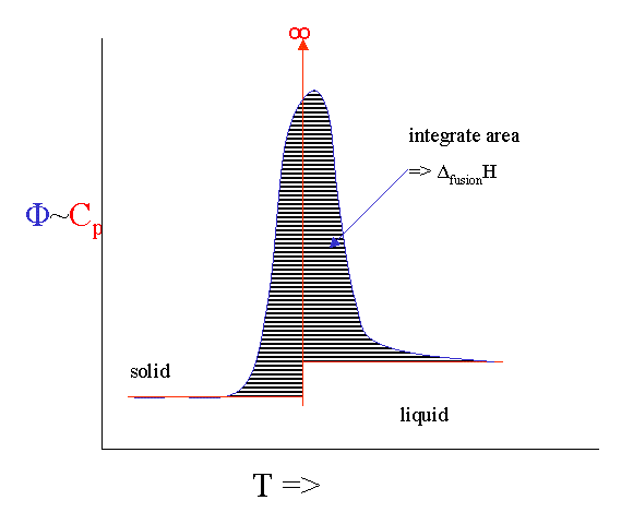
    However, there are number of serious broadening issues with the technique. If you melt something you will never get to see the infinite singularity of the heat capacity. Instead it broadens out into a peak. If you integrate the peak you get the ΔfusionH and the onset is calibrated to give you the melting point.
    alt
    The ideal heat capacity signal and its broadened DSC signal

    It is even possible to heat the sample with a rate that fluctuates with a little sine wave. This "Modulated DSC" version can even give you the (small) difference in \(C_p\) before and after the melting event.


    19.10: Relative Enthalpies Can Be Determined from Heat Capacity Data and Heats of Transition is shared under a CC BY-NC-SA 4.0 license and was authored, remixed, and/or curated by LibreTexts.

    • Was this article helpful?