3.2: Photon Echo

The photon echo experiment is most commonly used to distinguish static and dynamic linebroadening, and time-scales for energy gap fluctuations. The rephasing character of \(R_2\) and \(R_3\) allows you to separate homogeneous and inhomogeneous broadening.

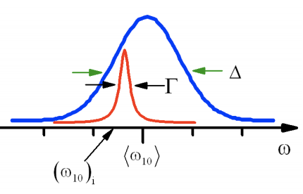
To demonstrate this let’s describe a photon echo experiment for an inhomogeneous lineshape, that is a convolution of a homogeneous line shape with width \(Γ\) with a static inhomogeneous distribution of width \(Δ\). Remember that linear spectroscopy cannot distinguish the two:

\[R(\tau)=|\mu_{ab}|^2e^{-i\omega_{ab}\tau-g(\tau)}-c.c. \label{4.2.1}\]

For an inhomogeneous distribution, we could average the homogeneous response, \(g(t)=\Gamma_{ba}t\), with an inhomogeneous distribution

\[R=\int d\omega_{ab}G\left(\omega_{ab}\right)R\left(\omega_{ab}\right) \label{4.2.2}\]

which we take to be Gaussian

\[G(\omega_{ba})=exp\left(-\frac{\left(\omega_{ba}-\langle\omega_{ba}\rangle\right)^2}{2\Delta^2}\right) \label{4.2.3}\]

Equivalently, since a convolution in the frequency domain is a product in the time domain, we can set

\[g(t)=\Gamma_{ba}t+\frac{1}{2}\Delta^2t^2 \label{4.2.4}\]

So for the case that \(\Delta \gt \Gamma\), the absorption spectrum is a broad Gaussian lineshape centered at the mean frequency \(\langle\omega_{ba}\rangle\) which just reflects the static distribution \(\Delta\) rather than the dynamics in \(\Gamma\).

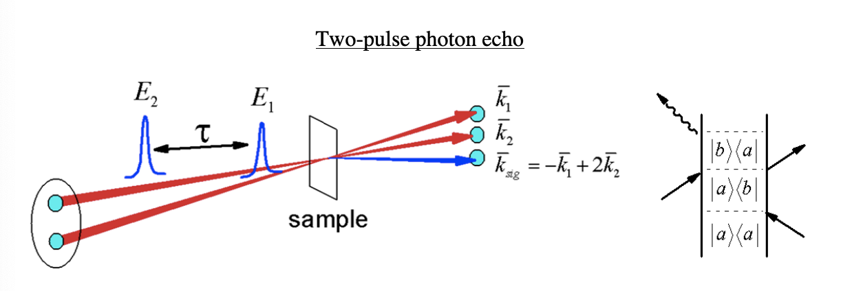
Now look at the experiment in which two pulses are crossed to generate a signal in the direction

\[k_{sig}=2k_2-k_1 \label{4.2.5}\]

This signal is a special case of the signal \((k_3+k_2-k_1)\) where the second and third interactions are both derived from the same beam. Both non-rephasing diagrams contribute here, but since both second and third interactions are coincident, \(\tau_2=0\) and \(R_2=R_3\). The nonlinear signal can be obtained by integrating the homogeneous response,

\[R^{(3)}(\omega_{ab})=|\mu_{ab}|^4p_ae^{-i\omega_{ab}(\tau_1-\tau_3)}e^{-\Gamma_{ab}(\tau_1+\tau_3)} \label{4.2.6}\]

over the inhomogeneous distribution as in eq. (4.2.2). This leads to

\[R^{(3)}=|\mu_{ab}|^4p_ae^{-i\langle\omega_{ab}\rangle(\tau_1-\tau_3)}e^{-\Gamma_{ab}(\tau_1+\tau_3)}e^{-(\tau_1-\tau_3)^2\Delta^2/2} \label{4.2.7}\]

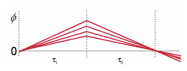
For \(\Delta \gt\gt \Gamma_{ab}\), \(R^{(3)}\) is sharply peaked at \(\tau_1=\tau_3\), i.e. \(e^{-(\tau_1-\tau_3)^2\Delta^2/2}\approx\delta(\tau_1-\tau_3)\). The broad distribution of frequencies rapidly dephases during \(\tau_1\), but is rephased (or refocused) during \(\tau_3\), leading to a large constructive enhancement of the polarization at \(\tau_1=\tau_3\). This rephasing enhancement is called an echo.

In practice, the signal is observed with a integrating intensity-level detector placed into the signal scattering direction. For a given pulse separation \(\tau\) (setting \(\tau_1=\tau\)), we calculated the integrated signal intensity radiated from the sample during \(\tau_3\) as

\[I_{sig}(\tau)=|E_{sig}|^2\propto\int_{-\infty}^{\infty}d\tau_3|P^{(3)}(\tau,\tau_3)|^2 \label{4.2.8}\]

In the inhomogeneous limit \((\Delta \gt\gt \Gamma_{ab})\), we find

\[I_{sig}(\tau)\propto|\mu_{ab}|^8e^{-4\Gamma_{ab}\tau} \label{4.2.9}\]

In this case, the only source of relaxation of the polarization amplitude at \(\tau_1=\tau_3\) is \(\Gamma_{ab}\). At this point inhomogeneity is removed and only the homogeneous dephasing is measured. The factor of four in the decay rate reflects the fact that damping of the initial coherence evolves over two periods \(\tau_1+\tau_3=2\tau\), and that an intensity level measurement doubles the decay rate of the polarization.