
3.2: Linear Approximations
- Page ID
- 106814

If you take a look at Equation \(3.1.5\) you will see that we can always approximate a function as \(a_0+a_1x\) as long as \(x\) is small. When we say ‘any function’ we of course imply that the function and all its derivatives need to be finite at \(x=0\). Looking at the definitions of the coefficients, we can write:
\[\label{eq1} f (x) \approx f(0) +f'(0)x\]
We call this a linear approximation because Equation \ref{eq1} is the equation of a straight line. The slope of this line is \(f'(0)\) and the \(y\)-intercept is \(f(0)\).
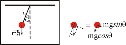
A fair question at this point is ‘why are we even talking about approximations?’ What is so complicated about the functions \(\sin{x}\), \(e^x\) or \(\ln{(x+1)}\) that we need to look for an approximation? Are we getting too lazy? To illustrate this issue, let’s consider the problem of the pendulum, which we will solve in detail in the chapter devoted to differential equations. The problem is illustrated in Figure \(\PageIndex{1}\), and those of you who took a physics course will recognize the equation below, which represents the law of motion of a simple pendulum. The second derivative refers to the acceleration, and the \(\sin \theta\) term is due to the component of the net force along the direction of motion. We will discuss this in more detail later in this semester, so for now just accept the fact that, for this system, Newton’s law can be written as:
\[\frac{d^2\theta(t)}{dt^2}+\frac{g}{l} \sin{\theta(t)}=0 \nonumber\]
This equation should be easy to solve, right? It has only a few terms, nothing too fancy other than an innocent sine function...How difficult can it be to obtain \(\theta(t)\)? Unfortunately, this differential equation does not have an analytical solution! An analytical solution means that the solution can be expressed in terms of a finite number of elementary functions (such as sine, cosine, exponentials, etc). Differential equations are sometimes deceiving in this way: they look simple, but they might be incredibly hard to solve, or even impossible! The fact that we cannot write down an analytical solution does not mean there is no solution to the problem. You can swing a pendulum and measure \(\theta(t)\) and create a table of numbers, and in principle you can be as precise as you want to be. Yet, you will not be able to create a function that reflects your numeric results. We will see that we can solve equations like this numerically, but not analytically. Disappointing, isn’t it? Well... don’t be. A lot of what we know about molecules and chemical reactions came from the work of physical chemists, who know how to solve problems using numerical methods. The fact that we cannot obtain an analytical expression that describes a particular physical or chemical system does not mean we cannot solve the problem numerically and learn a lot anyway!
But what if we are interested in small displacements only (that is, the pendulum swings close to the vertical axis at all times)? In this case, \(\theta<<1\), and as we saw \(\sin{\theta}\approx\theta\) (see Figure \(3.1.4\)). If this is the case, we have now:
\[\frac{d^2\theta(t)}{dt^2}+\frac{g}{l} \theta(t)=0 \nonumber\]
As it turns out, and as we will see in Chapter 2, in this case it is very easy to obtain the solution we are looking for:
\[\theta(t)=\theta(t=0)\cos \left((\frac{g}{l})^{1/2}t \right) \nonumber\]
This solution is the familiar ‘back and forth’ oscillatory motion of the pendulum you are familiar with. What you might have not known until today is that this solution assumes \(\sin{\theta}\approx\theta\) and is therefore valid only if \(\theta<<1\)!
There are lots of ‘hidden’ linear approximations in the equations you have learned in your physics and chemistry courses. You may recall your teachers telling you that a give equation is valid only at low concentrations, or low pressures, or low... you hopefully get the point. A pendulum is of course not particularly interesting when it comes to chemistry, but as we will see through many examples during the semester, oscillations, generally speaking, are. The example below illustrates the use of series to a problem involving diatomic molecules, but before discussing it we need to provide some background.
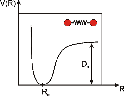
The vibrations of a diatomic molecule are often modeled in terms of the so-called Morse potential. This equation does not provide an exact description of the vibrations of the molecule under any condition, but it does a pretty good job for many purposes.
\[\label{morse}V(R)=D_e\left(1-e^{-k(R-R_e)}\right)^2\]
Here, \(R\) is the distance between the nuclei of the two atoms, \(R_e\) is the distance at equilibrium (i.e. the equilibrium bond length), \(D_e\) is the dissociation energy of the molecule, \(k\) is a constant that measures the strength of the bond, and \(V\) is the potential energy. Note that \(R_e\) is the distance at which the potential energy is a minimum, and that is why we call this the equilibrium distance. We would need to apply energy to separate the atoms even more, or to push them closer (Figure \(\PageIndex{2}\)).
At room temperature, there is enough thermal energy to induce small vibrations that displace the atoms from their equilibrium positions, but for stable molecules, the displacement is very small: \(R-R_e\rightarrow0\). In the next example we will prove that under these conditions, the potential looks like a parabola, or in mathematical terms, \(V(R)\) is proportional to the square of the displacement. This type of potential is called a ’harmonic potential’. A vibration is said to be simple harmonic if the potential is proportional to the square of the displacement (as in the simple spring problems you may have studied in physics).
Expand the Morse potential as a power series and prove that the vibrations of the molecule are approximately simple harmonic if the displacement \(R-R_e\) is small.
Solution
The relevant variable in this problem is the displacement \(R-R_e\), not the actual distance \(R\). Let’s call the displacement \(R-R_e=x\), and let’s rewrite Equation \ref{morse} as
\[\label{morse2}V(R)=D_e\left(1-e^{-kx}\right)^2\]
The goal is to prove that \(V(R) =cx^2\) (i.e. the potential is proportional to the square of the displacement) when \(x\rightarrow0\). The constant \(c\) is the proportionality constant. We can approach this in two different ways. One option is to expand the function shown in Equation \ref{morse2} around zero. This would be correct, but it but involve some unnecessary work. The variable \(x\) appears only in the exponential term, so a simpler option is to expand the exponential function, and plug the result of this expansion back in Equation \ref{morse2}. Let’s see how this works:
We want to expand \(e^{-kx}\) as \(a_0+a_1 x + a_2 x^2...a_n x^n\), and we know that the coefficients are \(a_n=\frac{1}{n!} \left( \frac{d^n f(x)}{dx^n} \right)_0.\)
The coefficient \(a_0\) is \(f(0)=1\). The first three derivatives of \(f(x)=e^{-kx}\) are
- \(f'(x)=-ke^{-kx}\)
- \(f''(x)=k^2e^{-kx}\)
- \(f'''(x)=-k^3e^{-kx}\)
When evaluated at \(x=0\) we obtain, \(-k, k^2, -k^3...\)
and therefore \(a_n=\frac{(-1)^n k^n}{n!}\) for \(n=0, 1, 2...\).
Therefore,
\[e^{-kx}=1-kx+k^2x^2/2!-k^3x^3/3!+k^4x^4/4!...\]
and
\[1-e^{-kx}=+kx-k^2x^2/2!+k^3x^3/3!-k^4x^4/4!...\]
From the last result, when \(x<<1\), we know that the terms in \(x^2, x^3...\) will be increasingly smaller, so \(1-e^{-kx}\approx kx\) and \((1-e^{-kx})^2\approx k^2x^2\).
Plugging this result in Equation \ref{morse2} we obtain \(V(R) \approx D_e k^2 x^2\), so we demonstrated that the potential is proportional to the square of the displacement when the displacement is small (the proportionality constant is \(D_e k^2\)). Therefore, stable diatomic molecules at room temperatures behave pretty much like a spring! (Don’t take this too literally. As we will discuss later, microscopic springs do not behave like macroscopic springs at all).