
28.8: Transition-State Theory Can Be Used to Estimate Reaction Rate Constants
- Page ID
- 14550
Transition State Theory
In Figure 28.8.1 , the point at which we evaluate or measure \(E_a\) serves as a dividing line (also called a dividing surface) between reactants and products. At this point, we do not have \(\text{A} + \text{B}\), and we do not have \(\text{C}\). Rather, what we have is an activated complex of some kind called a transition state between reactants and products. The value of the reaction coordinate at the transition state is denoted \(q^\ddagger\). Recall our notation \(\text{x}\) for the complete set of coordinates and momenta of all of the atoms in the system. Generally, the reaction coordinate \(q\) is a function \(q \left( \text{x} \right)\) of all of the coordinates and momenta, although typically, \(q \left( \text{x} \right)\) is a function of a subset of the coordinates and, possibly, the momenta.
As an example, let us consider two atoms \(\text{A}\) and \(\text{B}\) undergoing a collision. An appropriate reaction coordinate could simply be the distance \(r\) between \(\text{A}\) and \(\text{B}\). This distance is a function of the positions \(\textbf{r}_\text{A}\) and \(\textbf{r}_\text{B}\) of the two atoms, in that
\[q = r = \left| \textbf{r}_\text{A} - \textbf{r}_\text{B} \right| \label{20.24} \]
When \(\text{A}\) and \(\text{B}\) are molecules, such as proteins, \(q \left( \text{x} \right)\) is a much more complicated function of \(\text{x}\).
Now, recall that the mechanical energy \(\mathcal{E} \left( \text{x} \right)\) is given by
\[\mathcal{E} \left( \text{x} \right) = \sum_{i=1}^N \frac{\textbf{p}_i^2}{2m_1} + U \left( \textbf{r}_1, \ldots, \textbf{r}_N \right) \label{20.25} \]
and is a sum of kinetic and potential energies. Transition state theory assumes the following:
- The system is classical, and the time dependence of the coordinates and momenta is determined by Newton’s laws of motion \[m_i \ddot{\textbf{r}}_i = \textbf{F}_i \label{20.26} \]
- We start a trajectory obeying this equation of motion with an initial condition \(\text{x}\) that makes \(q \left( \text{x} \right) = q^\ddagger\) and such that \(\dot{q} \left( \text{x} \right) > 0\) so that the reaction coordinate proceeds initial to the right, i.e., toward products.
- We follow the motion \(\text{x}_t\) of the coordinates and momenta in time starting from this initial condition \(\text{x}\), which gives us a unique function \(\text{x}_t \left( \text{x} \right)\).
- If \(q \left( \text{x}_t \left( \text{x} \right) \right) > q^\ddagger\) at time \(t\), then the trajectory is designated as “reactive” and contributes to the reaction rate.
Define a function \(\theta \left( y \right)\), which is \(1\) if \(y \geq 0\) and \(0\) if \(y < 0\). The function \(\theta \left( y \right)\) is known as a step function.
We now define a flux of reactive trajectories \(k \left( t \right)\) using statistical mechanics
\[k \left( t \right) = \frac{1}{h Q_r} \int_{q \left( \text{x} \right) = q^\ddagger} d \text{x} \: e^{-\beta \mathcal{E} \left( \text{x} \right)} \left| \dot{q} \left( \text{x} \right) \right| \theta \left( q \left( \text{x}_t \left( \text{x} \right) \right) - q^\ddagger \right) \label{20.27} \]
where \(h\) is Planck’s constant. Here \(Q_r\) is the partition function of the reactants
\[Q_r = \int d \text{x} \: e^{-\beta \mathcal{E} \left( \text{x} \right)} \theta \left( q^\ddagger - q \left( \text{x} \right) \right) \label{20.28} \]
The meaning of Equation \(\ref{20.27}\) is an ensemble average over a canonical ensemble of the product \(\left| \dot{q} \left( \text{x} \right) \right|\) and \(\theta \left( q \left( \text{x}_t \left( \text{x} \right) \right) - q^\ddagger \right)\). The first factor in this product \(\left| \dot{q} \left( \text{x} \right) \right|\) forces the initial velocity of the reaction coordinate to be positive, i.e., toward products, and the step function \(\theta \left( q \left( \text{x}_t \left( \text{x} \right) \right) - q^\ddagger \right)\) requires that the trajectory of \(q \left( \text{x}_t \left( \text{x} \right) \right)\) be reactive, otherwise, the step function will give no contribution to the flux. The function \(k \left( t \right)\) in Equation \(\ref{20.27}\) is known as the reactive flux. In the definition of \(Q_r\) the step function \(\theta \left( q^\ddagger - q \left( \text{x} \right) \right)\) measures the total number of microscopic states on the reactive side of the energy profile.
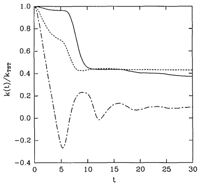
A plot of some examples of reactive flux functions \(k \left( t \right)\) is shown in Figure 28.8.2 . These functions are discussed in greater detail in J. Chem. Phys. 95, 5809 (1991). These examples all show that \(k \left( t \right)\) decays at first but then finally reaches a plateau value. This plateau value is taken to be the true rate of the reaction under the assumption that eventually, all trajectories that will become reactive will have done so after a sufficiently long time. Thus,
\[k = \underset{t \rightarrow \infty}{\text{lim}} k \left( t \right) \label{20.29} \]
gives the true rate constant. On the other hand, a common approximation is to take the value \(k \left( 0 \right)\) as an estimate of the rate constant, and this is known as the transition state theory approximation to \(k\), i.e.,
\[\begin{align} k^\text{(TST)} &= k \left( 0 \right) \\ &= \frac{1}{Q_r} \int_{q \left( \text{x} \right) = q^\ddagger} d \text{x} \: e^{-\beta \mathcal{E} \left( \text{x} \right)} \left| \dot{q} \left( \text{x} \right) \right| \theta \left( q \left( \text{x} \right) - q^\ddagger \right) \end{align} \label{20.30} \]
However, note that since we require \(\dot{q} \left( \text{x} \right)\) to initially be toward products, then by definition, at \(t = 0\), \(q \left( \text{x} \right) \geq q^\ddagger\), and the step function in the above expression is redundant. In addition, if \(\dot{q} \left( \text{x} \right)\) only depends on momenta (or velocities) and not actually on coordinates, which will be true if \(q \left( \text{x} \right)\) is not curvilinear (and is true for some curvilinear coordinates \(q \left( \text{x} \right)\)), and if \(q \left( \text{x} \right)\) only depends on coordinates, then Equation \(\ref{20.30}\) reduces to
\[k^\text{(TST)} = \frac{1}{h Q_r} \int d \text{x}_\textbf{p} e^{-\beta \sum_{i=1}^N \textbf{p}_i^2/2m_i} \left| \dot{q} \left( \textbf{p}_1, \ldots, \textbf{p}_N \right) \right| \int_{q \left( \textbf{r}_1, \ldots, \textbf{r}_N \right) = q^\ddagger} d \text{x}_\textbf{r} e^{-\beta U \left( \textbf{r}_1, \ldots, \textbf{r}_N \right)} \label{20.31} \]
The integral
\[Z^\ddagger = \int_{q \left( \textbf{r}_1, \ldots, \textbf{r}_N \right) = q^\ddagger} d \text{x}_\textbf{r} e^{-\beta U \left( \textbf{r}_1, \ldots, \textbf{r}_N \right)} \nonumber \]
counts the number of microscopic states consistent with the condition \(q \left( \textbf{r}_1, \ldots, \textbf{r}_N \right) = q^\ddagger\) and is, therefore, a kind of partition function, and is denoted \(Q^\ddagger\). On the other hand, because it is a partition function, we can derive a free energy \(\Delta F^\ddagger\) from it
\[F^\ddagger \propto -k_B T \: \text{ln} \: Z^\ddagger \label{20.32} \]
Similarly, if we divide \(Q_r\) into its ideal-gas and configurational contributions
\[Q_r = Q_r^\text{(ideal)} Z_r \label{20.33} \]
then we can take
\[Z_r = e^{-\beta F_r} \label{20.34} \]
where \(F_r\) is the free energy of the reactants. Finally, setting \(\dot{q} = p/\mu\), where \(\mu\) is the associated mass, and \(p\) is the corresponding momentum of the reaction coordinate, then, canceling most of the momentum integrals between the numerator and \(Q_r^\text{(ideal)}\), the momentum integral we need is
\[\int_0^\infty e^{-\beta p^2/2 \mu} \frac{p}{\mu} = k_B T \label{20.35} \]
which gives the final expression for the transition state theory rate constant
\[k^\text{(TST)} = \frac{k_B T}{h} e^{-\beta \left( F^\ddagger - F_r \right)} = \frac{k_B T}{h} e^{-\beta \Delta F^\ddagger} \label{20.36} \]
Figure 28.8.2 actually shows \(k \left( t \right)/ k^\text{(TST)}\), which must start at \(1\). As the figure shows, in addition, for \(t > 0\), \(k \left( t \right) < k^\text{(TST)}\). Hence, \(k^\text{(TST)}\) is always an upper bound to the true rate constant. Transition state theory assumes that any trajectory that initially moves toward products will be a reactive trajectory. For this reason, it overestimates the reaction rate. In reality, trajectories can cross the dividing surface several or many times before eventually proceeding either toward products or back toward reactants.
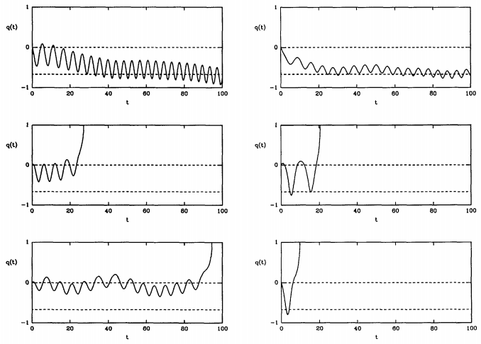
Figure 28.8.3 shows that one can obtain trajectories of both types. Here, the dividing surface lies at \(q = 0\). Left, toward \(q = -1\) is the reactant side, and right, toward \(q = 1\) is the product side. Because some trajectories return to reactants and never become products, the true rate is always less than \(k^\text{(TST)}\), and we can write
\[k = \kappa k^\text{(TST)} \label{20.37} \]
where the factor \(\kappa < 1\) is known as the transmission factor. This factor accounts for multiple recrossings of the dividing surface and the fact that some trajectories do not become reactive ones.