1.2: The Kinetic Model

The laws that describe the behavior of gases were well established long before anyone had developed a coherent model of the properties of gases. In this section, we introduce a theory that describes why gases behave the way they do. The theory we introduce can also be used to derive laws such as the perfect gas law from fundamental principles and the properties of individual particles.

One key property of the individual particles is their velocity. However, in a sample of many gas particles, the particles will likely have various velocities. Rather than list the velocity of each individual gas molecule, we can combine these individual velocities in several ways to obtain "collective" velocities that describe the sample as a whole. In the following example, three of these collective velocities are defined and calculated for a sample of gas consisting of only eight molecules.

Example \(\PageIndex{1}\): A Gas Sample with Few Molecules

The speeds of eight molecules were found to be 1.0, 4.0, 4.0, 6.0, 6.0, 6.0, 8.0, and 10.0 m/s. Calculate their average speed (\(v_{\rm avg}\)) root mean square speed (\(v_{\rm rms}\)), and most probable speed (\(v_{\rm mp}\)).

• average speed (\(v_{\rm avg}\)) = the sum of all the speeds divided by the number of molecules
• root-mean square speed (\(v_{\rm rms}\)) = the square root of the sum of the squared speeds divided by the number of molecules
• most probable speed (\(v_{\rm mp}\)) = the speed at which the greatest number of molecules is moving

Solution:

The average speed:

\[v_{\rm avg}=\rm\dfrac{(1.0+4.0+4.0+6.0+6.0+6.0+8.0+10.0)\;m/s}{8}=5.6\;m/s\]

The root-mean square speed:

\[v_{\rm rms}=\rm\sqrt{\dfrac{(1.0^2+4.0^2+4.0^2+6.0^2+6.0^2+6.0^2+8.0^2+10.0^2)\;m^2/s^2}{8}}=6.2\;m/s\]

The most probable speed:

Of the eight molecules, three have speeds of 6.0 m/s, two have speeds of 4.0 m/s, and the other three molecules have different speeds. Hence

\[v_{\rm mp}=6.0\, m/s.\]

The calculations carried out in Example \(\PageIndex{1}\) become cumbersome as the number of molecules in the sample of gas increases. Thus, a more efficient way to determine the various collective velocities for a gas sample containing a large number of molecules is required.

A Molecular Description of Pressure and Molecular Speed

The kinetic molecular theory of gases explains the laws that describe the behavior of gases. Developed during the mid-19th century by several physicists, including the Austrian Ludwig Boltzmann (1844–1906), the German Rudolf Clausius (1822–1888), and the Scotsman James Clerk Maxwell (1831–1879), this theory is based on the properties of individual particles as defined for an ideal gas and the fundamental concepts of physics. Thus the kinetic molecular theory of gases provides a molecular explanation for observations that led to the development of the ideal gas law. The kinetic molecular theory of gases is based on the following five postulates:

1. A gas is composed of a large number of particles called molecules (whether monatomic or polyatomic) that are in constant random motion.
2. Because the distance between gas molecules is much greater than the size of the molecules, the volume of the molecules is negligible.
3. Intermolecular interactions, whether repulsive or attractive, are so weak that they are also negligible.
4. Gas molecules collide with one another and with the walls of the container, but these collisions are perfectly elastic; that is, they do not change the average kinetic energy of the molecules.
5. The average kinetic energy of the molecules of any gas depends on only the temperature, and at a given temperature, all gaseous molecules have exactly the same average kinetic energy.

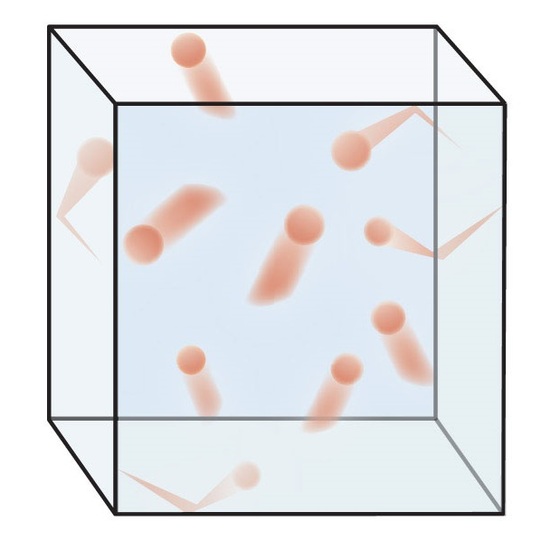
Figure \(\PageIndex{1}\): Visualizing molecular motion. Molecules of a gas are in constant motion and collide with one another and with the container wall.

Although the molecules of real gases have nonzero volumes and exert both attractive and repulsive forces on one another, for the moment we will focus on how the kinetic molecular theory of gases relates to the properties of gases we have been discussing. In Topic 1C, we explain how this theory must be modified to account for the behavior of real gases.

Postulates 1 and 4 state that gas molecules are in constant motion and collide frequently with the walls of their containers. The collision of molecules with their container walls results in a momentum transfer (impulse) from molecules to the walls (Figure \(\PageIndex{2}\)).

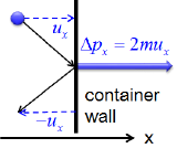
Figure \(\PageIndex{2}\): Note: In this figure, the symbol \(u\) is used to represent velocity. In the rest of this text, velocity will be represented with the symbol \(v\). Momentum transfer (Impulse) from a molecule to the container wall as it bounces off the wall. Momentum transfer (\(\Delta \rho_x\)) for an elastic collision is equal to m\(\Delta v_x\), where m is the mass of the molecule and \(\Delta v_x\) is the change in the \(x\) component of the molecular velocity (\(v_{x_{final}}-v_{x_{initial}})\).The wall is perpendicular to \(x\) axis. Since the collisions are elastic, the molecule bounces back with the same velocity in the opposite direction, and \(\Delta v_x\) equals \(2v_x\).

The momentum transfer to the wall perpendicular to \(x\) axis as a molecule with an initial velocity \(v_x\) in \(v\) direction hits is expressed as:

\[\rm momentum\; transfer_x\;= \Delta \rho_x = m\Delta v_x = 2mv_x \label{1.2.1}\]

The collision frequency, a number of collisions of the molecules to the wall per unit area and per second, increases with the molecular speed and the number of molecules per unit volume.

\[f\propto (v_x) \times \Big(\dfrac{N}{V}\Big) \label{1.2.2}\]

The pressure the gas exerts on the wall is expressed as the product of impulse and the collision frequency.

\[P\propto (2mv_x)\times(v_x)\times\Big(\dfrac{N}{V}\Big)\propto \Big(\dfrac{N}{V}\Big)mv_x^2 \label{1.2.3}\]

At any instant, however, the molecules in a gas sample are traveling at different speed. Therefore, we must replace \(v_x^2\) in the expression above with the average value of \(v_x^2\), which is denoted by \(\bar{v_x^2}\). The overbar designates the average value over all molecules.

The exact expression for pressure is given as :

\[P=\dfrac{N}{V}m\bar{v_x^2} \label{1.2.4}\]

Finally, we must consider that there is nothing special about \(x\) direction. We should expect that \(\bar{v_x^2}= \bar{v_y^2}=\bar{v_z^2}=\dfrac{1}{3}\bar{v^2}\). Here the quantity \(\bar{v^2}\) is called the mean-square speed defined as the average value of square-speed (\(v^2\)) over all molecules. Since \(v^2=v_x^2+v_y^2+v_z^2\) for each molecule, \(\bar{v^2}=\bar{v_x^2}+\bar{v_y^2}+\bar{v_z^2}\). By substituting \(\dfrac{1}{3}\bar{v^2}\) for \(\bar{v_x^2}\) in the expression above, we can get the final expression for the pressure:

\[P=\dfrac{1}{3}\dfrac{N}{V}m\bar{v^2} \label{1.2.5}\]

Because volumes and intermolecular interactions are negligible, postulates 2 and 3 state that all gaseous particles behave identically, regardless of the chemical nature of their component molecules. This is the essence of the ideal gas law, which treats all gases as collections of particles that are identical in all respects except mass. Postulate 2 also explains why it is relatively easy to compress a gas; you simply decrease the distance between the gas molecules.

Postulate 5 provides a molecular explanation for the temperature of a gas. Postulate 5 refers to the average translational kinetic energy of the molecules of a gas,

\[\epsilon = m\bar{v^2}/2\label{1.2.6}\]

By rearranging equation \(\ref{1.2.5}\) and substituting in equation \(\ref{1.2.6}\), we obtain

\[PV = \dfrac{1}{3} N m \bar{v^2} = \dfrac{2}{3} N \epsilon \label{1.2.7}\]

The 2/3 factor in the proportionality reflects the fact that velocity components in each of the three directions contributes ½ kT to the kinetic energy of the particle. The average translational kinetic energy is directly proportional to temperature:

\[\epsilon = \dfrac{3}{2} kT \label{1.2.8}\]

in which the proportionality constant \(k\) is known as the Boltzmann constant. Substituting Equation \(\ref{1.2.8}\) into Equation \(\ref{1.2.7}\) yields

\[ PV = \left( \dfrac{2}{3}N \right) \left( \dfrac{3}{2}kT \right) =NkT \label{1.2.9}\]

The Boltzmann constant \(k\) is just the gas constant per molecule, so if N is chosen as Avogadro's number, \(N_A\), then \(N_Ak\) is R, the gas constant per mole. Thus, for n moles of particles, the Equation \(\ref{1.2.9}\) becomes

\[ PV = nRT \label{1.2.10}\]

which is the perfect gas law.

As noted in Example \(\PageIndex{1}\) , the root-mean square speed (\(v_{\rm rms}\)) is the square root of the sum of the squared speeds divided by the number of particles:

\[v_{\rm rms}=\sqrt{\bar{v^2}}=\sqrt{\dfrac{v_1^2+v_2^2+\cdots v_N^2}{N}} \label{1.2.11}\]

where \(N\) is the number of particles and \(v_i\) is the speed of particle \(i\).

The \(v_{\rm rms}\) for a sample containing a large number of molecules can be obtained by combining equations \(\ref{1.2.7}\) and \(\ref{1.2.8}\) in a slightly different fashion than that used to obtain equation \(\ref{1.2.10}\):

\[PV=\dfrac{1}{3} N m \bar{v^2} = \dfrac{2}{3} N \epsilon \tag{1.2.7}\]

\[\epsilon = \dfrac{3}{2} kT \tag{1.2.8}\]

\[\dfrac{1}{3} N m \bar{v^2}= \left(\dfrac{2}{3}\right)\left(\dfrac{3}{2}\right) NkT \label{1.2.12}\]

\[\dfrac{1}{3} N m \bar{v^2}= NkT \label{1.2.13}\]

\[ N m \bar{v^2}= 3NkT \label{1.2.14}\]

If N is chosen to be Avogadro's number, \(N_A\), then \(N_Am = M\), the molar mass, and \(N_Ak = R\), the gas constant per mole,

\[\bar{v^2} = \dfrac{3RT}{M} \label{1.2.15}\]

\[v_{\rm rms}=\sqrt{\bar{v^2}}=\sqrt{\dfrac{3RT}{M}} \label{1.2.16}\]

In Equation \(\ref{1.2.16}\), \(v_{\rm rms}\) has units of meters per second; consequently, the units of molar mass \(M\) are kilograms per mole, temperature \(T\) is expressed in kelvins, and the ideal gas constant \(R\) has the value 8.3145 J/(K•mol). Equation \(\ref{1.2.16}\) shows that \(v_{\rm rms}\) of a gas is proportional to the square root of its Kelvin temperature and inversely proportional to the square root of its molar mass. The root mean-square speed of a gas increase with increasing temperature. At a given temperature, heavier gas molecules have slower speeds than do lighter ones.

Example \(\PageIndex{2}\):

What is the root mean-square speed for \(\rm O_2\) molecules at 25ºC?

Given: Temperature in ºC, type of molecules, ideal gas gas constant

Asked for: \(v_{\rm rms}\), the root mean-square speed

Strategy:

Convert temperature to kelvins:

\(\rm T\; (in\; kelvin) = (25ºC + 273ºC)\dfrac{1\; K}{1\; ºC} = 298\; K\)

Convert molar mass of \(\rm O_2\) molecules to kg per mole:

\(\rm M\; (in\; \dfrac{kg}{mole}) = 32.00\dfrac{g}{mole}\rm x\dfrac{1\; kg}{1000\; g}=0.03200\dfrac{kg}{mole}\)

Use equation \(\ref{1.2.16}\) to calculate the rms speed.

Solution

\(v_{\rm rms_{\rm O_2}}= \sqrt{\dfrac{3\rm (8.3145\dfrac{J}{K·mole})(298.15\; K)}{\rm 0.03200\dfrac{kg}{mole}}}=482\dfrac{m}{s}\)

Exercise \(\PageIndex{2}\)

What is the root mean-square speed for \(\rm Cl_2\) molecules at 25ºC?

\(v_{\rm rms_{\rm Cl_2}}= 324\dfrac{m}{s}\)

Many molecules, many velocities

At temperatures above absolute zero, all molecules are in motion. In the case of a gas, this motion consists of straight-line jumps whose lengths are quite great compared to the dimensions of the molecule. Although we can never predict the velocity of a particular individual molecule, the fact that we are usually dealing with a huge number of them allows us to know what fraction of the molecules have kinetic energies (and hence velocities) that lie within any given range.

The trajectory of an individual gas molecule consists of a series of straight-line paths interrupted by collisions. What happens when two molecules collide depends on their relative kinetic energies; in general, a faster or heavier molecule will impart some of its kinetic energy to a slower or lighter one. Two molecules having identical masses and moving in opposite directions at the same speed will momentarily remain motionless after their collision.

If we could measure the instantaneous velocities of all the molecules in a sample of a gas at some fixed temperature, we would obtain a wide range of values. A few would be zero, and a few would be very high velocities, but the majority would fall into a more or less well defined range. We might be tempted to define an average velocity for a collection of molecules, but here we would need to be careful: molecules moving in opposite directions have velocities of opposite signs. Because the molecules are in a gas are in random thermal motion, there will be just about as many molecules moving in one direction as in the opposite direction, so the velocity vectors of opposite signs would all cancel and the average velocity would come out to zero. Since this answer is not very useful, we need to do our averaging in a slightly different way.

The proper treatment is to average the squares of the velocities, and then take the square root of this value to obtain the root-mean square velocity (\(v_{\rm rms}\)), which is what we developed above. This velocity describes the gas sample as a whole, but it does not tell us about the range of velocities possible, nor does it tell us the distribution of velocities. To obtain a more complete description of how many gas molecules are likely to be traveling at a given velocity range we need to make use of the Maxwell-Boltzmann distribution law.

The Boltzmann Distribution

If we were to plot the number of molecules whose velocities fall within a series of narrow ranges, we would obtain a slightly asymmetric curve known as a velocity distribution. The peak of this curve would correspond to the most probable velocity. This velocity distribution curve is known as the Maxwell-Boltzmann distribution, but is frequently referred to only by Boltzmann's name. The Maxwell-Boltzmann distribution law was first worked out around 1850 by James Maxwell, and several years later Ludwig Boltzmann put the relation on a sounder theoretical basis and simplified the mathematics somewhat. Boltzmann pioneered the application of statistics to the physics and thermodynamics of matter, and was an ardent supporter of the atomic theory of matter at a time when it was still not accepted by many of his contemporaries.

The Maxwell-Boltzmann distribution is used to determine how many molecules are moving between velocities \(v\) and \(v + dv\). Assuming that the one-dimensional distributions are independent of one another, that the velocity in the y and z directions does not affect the x velocity, for example, the Maxwell-Boltzmann distribution is given by

\[ \dfrac{dN}{N} = \sqrt{\dfrac{m}{2\pi kT}} \exp\left [\dfrac{-mv^2}{2k T}\right] dv \label{1.2.17}\]

where

• \(dN/N\) is the fraction of molecules moving at velocity \(v\) to \(v + dv\),
• \(m\) is the mass of the molecule,
• \(k\) is the Boltzmann constant, and
• \(T\) is the absolute temperature.¹

Additionally, the function can be written in terms of the scalar quantity speed \(v\) instead of the vector quantity velocity. This form of the function defines the distribution of the gas molecules moving at different speeds, between \(v_1\) and \(v_2\), thus

\[f(v)=4\pi v^2 \left (\dfrac{m}{2\pi k T} \right)^{3/2}exp\left [\frac{-mv^2}{2kT}\right] \label{1.2.18}\]

Note

The speed of an individual gas particle is:

\[v =v_x+ v_y + v_z\]

Thus, the kinetic energy of the gas particle is:

\[\epsilon = \dfrac{1}{2}mv_x^2 + \dfrac{1}{2}mv_y^2 + \dfrac{1}{2}mv_z^2\label{1.2.19}\]

The Boltzmann distribution assumes that the portion of molecules with a specific velocity is proportional to an exponential function of the kinetic energy of the molecules:

\[f(v) = \left(\rm constant\right)exp\left [\dfrac{-mv^2}{2kT}\right] \label{1.2.20}\]

When the x, y, and z components of the velocities are taken into account, the equation becomes:

\[f(v) = \left(\rm constant\right) \times exp\left [\dfrac{-mv_x^2}{2kT}\right] \times exp\left [\dfrac{-mv_y^2}{2kT}\right] \times exp\left [\dfrac{-mv_z^2}{2kT}\right] \label{1.2.21}\]

This equation can be simplified and separated to:

\[f(v_x) = K_x exp\left[\dfrac{-mv_x^2}{2kT}\right]\label{1.2.22}\]

\[f(v_y) = K_y exp\left[\dfrac{-mv_y^2}{2kT}\right]\label{1.2.23}\]

\[f(v_z) = K_z exp\left[\dfrac{-mv_z^2}{2kT}\right]\label{1.2.24}\]

The constant, K, can be determined for each equation by assuming that the velocity along the given component must be between -\(\infty\) and +\(\infty\). Thus

\[\int_{-\infty}^{+\infty} \! f(v_x) \, \mathrm{d}v_x = 1\label{1.2.25}\]

To solve for \(f(v_x)\), we substitute equation \(\ref{1.2.22}\) into Equation \(\ref{1.2.25}\) to get

\[1 = K_x\int_{-\infty}^{+\infty} \! exp\left[\dfrac{-mv_x^2}{2kT}\right] \, \mathrm{d}v_x = K_x \left(\dfrac{2\pi kT}{m}\right)^{1/2}\label{1.2.26}\]

If

\[1 = K_x \left(\dfrac{2\pi kT}{m}\right)^{1/2}\label{1.2.27}\]

then

\[K_x = \left(\dfrac{m}{2\pi kT}\right)^{1/2}\label{1.2.28}\]

and

\[f(v_x) = \left(\dfrac{m}{2\pi kT}\right)^{1/2}\times exp\left[\dfrac{-mv_x^2}{2kT}\right] \label{1.2.29}\]

Combining all three components gives us:

\[f(v_x)f(v_y)f(v_z) = \left(\dfrac{m}{2\pi kT}\right)^{3/2}\times exp\left[\dfrac{-mv_x^2}{2kT}\right] \times exp\left [\dfrac{-mv_y^2}{2kT}\right] \times exp\left [\dfrac{-mv_z^2}{2kT}\right] \mathrm{d}v_x\mathrm{d}v_y\mathrm{d}v_z \label{1.2.30}\]

If we define

\[v^2 =v_x^2+ v_y^2 + v_z^2\label{1.2.31}\]

then Equation \(\ref{1.2.30}\) can be written as

\[f(v_x)f(v_y)f(v_z) = \left(\dfrac{m}{2\pi kT}\right)^{3/2}\times exp\left [\dfrac{-mv^2}{2kT}\right] \mathrm{d}v_x\mathrm{d}v_y\mathrm{d}v_z \label{1.2.32}\]

To determine the likelihood that a molecule has a speed in the range between \(v\) and \(v + dv\) we evaluate the probability that the molecule has a speed that is anywhere on the surface of a sphere of radius \(v\) by adding all the probabilities that it is in the volume element \(\mathrm{d}v_x\mathrm{d}v_y\mathrm{d}v_z\) at a distance \(v\) from the center. Thus, we assume a velocity space with coordinates (\(v_x,v_y,v_z\)), and also assume that the volume in velocity space is a spherical shell with radius \(v\), a surface area of \(4\pi v^2\), and a thickness of \(\mathrm{d}v\). This results in the volume being \(4\pi v^2\mathrm{d}v\).

The probability can be written as:

\[f(v)\mathrm{d}v = 4\pi v^2\mathrm{d}v\left(\dfrac{m}{2\pi kT}\right)^{3/2}\times exp\left [\dfrac{-mv^2}{2kT}\right] \label{1.2.33}\]

Upon rearrangement we get Equation \(\ref{1.2.18}\):

\[f(v)=4\pi v^2 \left (\dfrac{m}{2\pi kT} \right)^{3/2}exp\left [\frac{-mv^2}{2kT}\right] \tag{1.2.18}\]

Finally, the Maxwell-Boltzmann distribution can be used to determine the distribution of the kinetic energy of for a set of molecules. The distribution of the kinetic energy is identical to the distribution of the speeds for a certain gas at any temperature.² The Maxwell-Boltzmann distribution is a probability distribution and just like any such distribution, can be characterized in a variety of ways including.

• Average Speed: The average speed is the sum of the speeds of all of the particles divided by the number of particles.
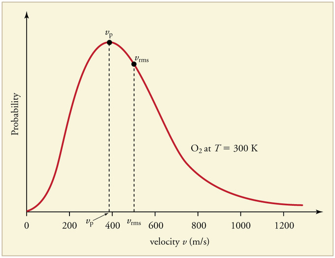
• Most Probable Speed: The most probable speed is the speed associated with the highest point in the Maxwell distribution. Only a small fraction of particles might have this speed, but it is more likely than any other speed.
• Width of the Distribution: The width of the distribution characterizes the most likely range of speeds for the particles. One measure of the width is the Full Width at Half Maximum (FWHM). To determine this value, find the height of the distribution at the most probable speed (this is the maximum height of the distribution). Divide the maximum height by two to obtain the half height, and locate the two speeds in the distribution that have this half-height value. One speed will be greater than the most probable speed and the other speed will be smaller. The full width is the difference between the two speeds at the half-maximum value.

Velocity distributions depend on temperature and mass

Higher temperatures allow a larger fraction of molecules to acquire greater amounts of kinetic energy, causing the Boltzmann plots to spread out. Figure \(\PageIndex{4}\) shows how the Maxwell-Boltzmann distribution is affected by temperature. At lower temperatures, the molecules have less energy. Therefore, the speeds of the molecules are lower and the distribution has a smaller range. As the temperature of the molecules increases, the distribution flattens out. Because the molecules have greater energy at higher temperature, the molecules are moving faster.

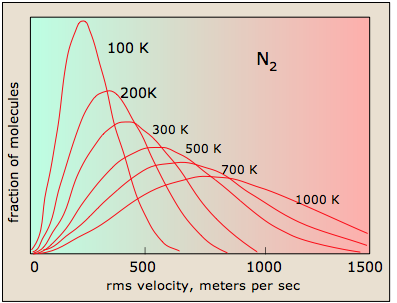
Figure \(\PageIndex{3}\): The Maxwell Distribution as a function of temperature for nitrogen molecules

Notice how the left ends of the plots are anchored at zero velocity (there will always be a few molecules that happen to be at rest.) As a consequence, the curves flatten out as the higher temperatures make additional higher-velocity states of motion more accessible. The area under each plot is the same for a constant number of molecules.

All molecules have the same kinetic energy (mv²/2) at the same temperature, so the fraction of molecules with higher velocities will increase as m, and thus the molecular weight, decreases. Figure \(\PageIndex{4}\) shows the dependence of the Maxwell-Boltzmann distribution on molecule mass. On average, heavier molecules move more slowly than lighter molecules. Therefore, heavier molecules will have a smaller speed distribution, while lighter molecules will have a speed distribution that is more spread out.

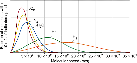
Figure \(\PageIndex{4}\): The speed probability density functions of the speeds of a few gases at a temperature of 298.15 K ). The y-axis is in s/m so that the area under any section of the curve (which represents the probability of the speed being in that range) is dimensionless.

The Maxwell-Boltzmann equation, which forms the basis of the kinetic theory of gases, defines the distribution of speeds for a gas at a certain temperature. From this distribution function, the most probable speed, the average speed, and the root-mean-square speed can be derived.

Related Speed Expressions

Four speed expressions can be derived from the Maxwell-Boltzmann distribution:

• the root-mean square speed,
• the most probable speed,
• the average speed, and
• the average relative speed.

The root-mean-square speed, derived above, is square root of the average speed-squared.

\[ v_{rms}= \sqrt{\bar{v^2}} = \sqrt {\dfrac {3RT}{M}} \tag{1.2.16}\]

where

• \(R\) is the gas constant,
• \(T\) is the absolute temperature and
• \(M\) is the molar mass of the gas.

The most probable speed is the maximum value on the distribution plot (Figure \(\PageIndex{5}\)). This is established by finding the velocity when the derivative of Equation \(\ref{1.2.18}\) is zero

\[\dfrac{df(v)}{dv} = 0 \label{1.2.35}\]

which is

\[ v_{mp}=\sqrt {\dfrac {2RT}{M}} \label{1.2.36}\]

\[v_{mp}=\sqrt {\dfrac{2}{3}}\; v_{rms}\label{1.2.37}\]

Figure \(\PageIndex{5}\): The Maxwell-Boltzmann distribution is shifted to higher speeds and is broadened at higher temperatures.Image used with permission from OpenStax. The speed at the top of the curve is called the most probable speed because the largest number of molecules have that speed.

The average speed is the sum of the speeds of all the molecules divided by the number of molecules.

\[v_{avg}= \bar{v} = \int_0^{\infty} v f(v) dv \label{1.2.38}\]

Recall from equation \(\ref{1.2.18}\) that

\[f(v)=4\pi v^2 \left (\dfrac{m}{2\pi kT} \right)^{3/2}exp\left [\frac{-mv^2}{2kT}\right] \tag{1.2.18}\]

Thus, equation \(\ref{1.2.38}\) becomes

\[v_{avg}= \bar{v} = 4\pi \left (\dfrac{m}{2\pi kT} \right)^{3/2} \int_0^{\infty} v^3exp\left [\frac{-mv^2}{2kT}\right] dv \label{1.2.39}\]

Upon solving the integral, we obtain

\[v_{avg}= \bar{v} = 4\pi \left (\dfrac{m}{2\pi kT} \right)^{3/2}\times \dfrac{1}{2}\left (\dfrac{2RT}{M} \right)^{1/2} = \left(\dfrac{8RT}{\pi M} \right)^{1/2}\label{1.2.40}\]

\[v_{avg}= \left(\dfrac{8RT}{\pi M} \right)^{1/2} \label{1.2.41}\]

\[v_{avg}=\left (\dfrac{8}{3\pi} \right)^{1/2}\; v_{rms}\label{1.2.42}\]

The rms speed and the average speed do not differ greatly (typically by less than 10%). The distinction is important, however, because the rms speed is the speed of a gas particle that has average kinetic energy. Particles of different gases at the same temperature have the same average kinetic energy, not the same average speed. In contrast, the most probable speed (\(v_{mp}\)) is the speed at which the greatest number of particles is moving. If the average kinetic energy of the particles of a gas increases linearly with increasing temperature, then Equation \(\ref{1.2.16}\) tells us that the rms speed must also increase with temperature because the mass of the particles is constant. At higher temperatures, therefore, the molecules of a gas move more rapidly than at lower temperatures, and \(v_{mp}\) increases. It is important to remember that the rms speed is always faster than the average speed, which is always greater than the most probable speed:

\[v_{rms} > v_{avg} > v_{mp} \label{1.2.43}\]

The average relative speed is used to calculate the collision frequency between two gas molecules in a low density sample of a perfect gas⁴. The average relative speed \(v_{\rm rel}\) is the average speed with which two molecules approach each other. The derivation of \(v_{\rm rel}\) is complicated by the fact that one of the molecules can approach the second molecule from any direction. Thus there can be a head-on collision, a glancing blow from an acute or obtuse angle, or an overtaking of a slower molecule by a faster molecule. In very simple terms,

\[v_{\rm rel}=v_1 - v_2\label{1.2.44}\]

After taking into account all of the possible angles of collision, and the fact that the molecules may have different masses, the net result is

\[v_{\rm rel} =\left (\dfrac{8kT}{\pi\mu} \right)^{1/2}\label{1.2.45}\]

where \(\mu\) is the reduced mass of the colliding pair of molecules:

\[\mu= \dfrac{ m_A m_B}{m_A + m_B}\label{1.2.46}\]

If the colliding molecules are the same kind, then

\[\mu= \dfrac{ m_A m_B}{m_A + m_B} = \dfrac{m}{2}\label{1.2.47}\]

and

\[v_{\rm rel} = \left (\dfrac{16kT}{\pi m} \right)^{1/2} = \sqrt{2}\; v_{\rm avg}\label{1.2.48}\]

Exercise \(\PageIndex{2}\) A Large Sample

1. Using the Maxwell-Boltzmann function, calculate the fraction of argon gas molecules with a speed of 305 m/s at 500 K.
2. If the system in problem 1 has 0.46 moles of argon gas, how many molecules have the speed of 305 m/s?
3. Calculate the values of \(v_{\rm mp}\), \(v_{\rm avg}\), and \(v_{\rm rms}\) for xenon gas at 298 K.
4. What will have a larger speed distribution, helium at 500 K or argon at 300 K? Helium at 300 K or argon at 500 K? Argon at 400 K or argon at 1000 K?

Answers

1. 0.00141
2. \(3.92 \times 10^{20}\) argon molecules
3. v_mp = 194.27 m/s, v_avg = 219.21 m/s, v_rms = 237.93 m/s
4. Hint: Use the related speed expressions to determine the distribution of the gas molecules: helium at 500 K. helium at at 300 K. argon at 1000 K.

The Relationships among Pressure, Volume, and Temperature

We now describe how the kinetic molecular theory of gases explains some of the important relationships we have discussed previously.

• Pressure versus Volume: At constant temperature, the kinetic energy of the molecules of a gas and hence the rms speed remain unchanged. If a given gas sample is allowed to occupy a larger volume, then the speed of the molecules does not change, but the density of the gas (number of particles per unit volume) decreases, and the average distance between the molecules increases. Hence the molecules must, on average, travel farther between collisions. They therefore collide with one another and with the walls of their containers less often, leading to a decrease in pressure. Conversely, increasing the pressure forces the molecules closer together and increases the density, until the collective impact of the collisions of the molecules with the container walls just balances the applied pressure.
• Volume versus Temperature: Raising the temperature of a gas increases the average kinetic energy and therefore the rms speed (and the average speed) of the gas molecules. Hence as the temperature increases, the molecules collide with the walls of their containers more frequently and with greater force. This increases the pressure, unless the volume increases to reduce the pressure, as we have just seen. Thus an increase in temperature must be offset by an increase in volume for the net impact (pressure) of the gas molecules on the container walls to remain unchanged.
• Pressure of Gas Mixtures: Postulate 3 of the kinetic molecular theory of gases states that gas molecules exert no attractive or repulsive forces on one another. If the gaseous molecules do not interact, then the presence of one gas in a gas mixture will have no effect on the pressure exerted by another, and Dalton’s law of partial pressures holds.

Example \(\PageIndex{3}\)

The temperature of a 4.75 L container of N₂ gas is increased from 0°C to 117°C. What is the qualitative effect of this change on the

1. average kinetic energy of the N₂ molecules?
2. \(v_{\rm rms}\) of the N₂ molecules?
3. \(v_{\rm avg}\) of the N₂ molecules?
4. impact of each N₂ molecule on the wall of the container during a collision with the wall?
5. total number of collisions per second of N₂ molecules with the walls of the entire container?
6. number of collisions per second of N₂ molecules with each square centimeter of the container wall?
7. pressure of the N₂ gas?

Answers:

1. Increasing the temperature increases the average kinetic energy of the N₂ molecules.
2. An increase in average kinetic energy can be due only to an increase in the rms speed of the gas particles.
3. If the \(v_{\rm rms}\) of the N₂ molecules increases, the \(v_{\rm avg}\) also increases.
4. If, on average, the particles are moving faster, then they strike the container walls with more energy.
5. Because the particles are moving faster, they collide with the walls of the container more often per unit time.
6. The number of collisions per second of N₂ molecules with each square centimeter of container wall increases because the total number of collisions has increased, but the volume occupied by the gas and hence the total area of the walls are unchanged.
7. The pressure exerted by the N₂ gas increases when the temperature is increased at constant volume, as predicted by the ideal gas law.

Collisions

Collisional frequency is the average rate at which two reactants collide for a given system, and is used to express the average number of collisions per unit of time in a defined system.

Background and Overview

To fully understand how the collisional frequency equation is derived, consider a simple system (a jar full of helium) and add each new concept in a step-by-step fashion. Also, although technically these statements are false, the following assumptions are used when deriving and calculating the collisional frequency:

• All molecules travel through space in straight lines.
• All molecules are hard, solid spheres.
• The reaction of interest is between only two molecules.
• Collisions are hit or miss only. They occur when distance between the center of the two reactants is less than or equal to the sum of their respective radii. Even if the two molecules barely miss each other, it is still considered a complete miss. The two molecules do not interact (in reality, their electron clouds would interact, but this has no bearing on the equation).

A Single Molecule Moving

In determining the collisional frequency for a single molecule, \(Z_i\), picture a jar filled with helium atoms. These atoms collide by hitting other helium atoms within the jar. If every atom except one is frozen and the number of collisions in one minute is counted, the collisional frequency (per minute) of a single atom of helium within the container could be determined. This is the basis for the equation.

\[Z_i = \dfrac{(Volume \; of \; Collisional \; Cylinder) (Density)}{Time}\label{1.2.49}\]

Figure \(\PageIndex{6}\): The collisional cylinder of a single moving molecule moving through space.

While the helium atom is moving through space, it sweeps out a collisional cylinder, as shown above. If the center of another helium atom is present within the cylinder, a collision occurs. The length of the cylinder is the helium atom's mean relative speed, \(\bar c_{\rm rel}\) in the above figure) \(v_{\rm rel} = \sqrt{2}\; v_{\rm avg}\), multiplied by change in time, \(\Delta{t}\). The mean relative speed is used instead of average speed because, in reality, the other atoms are moving and this factor accounts for some of that. The area of the cylinder face is the helium atom's collisional cross section, \(\sigma = \pi d^2\)

Although collision will most likely change the direction an atom moves, it does not affect the volume of the collisional cylinder, which is due to density being uniform throughout the system. Therefore, an atom has the same chance of colliding with another atom regardless of direction as long as the distance traveled is the same.

\[Volume \; of \; Collisional \; Cylinder = \sigma v_{\rm rel}\Delta{t}\label{1.2.50}\]

Density

Next, account must be taken of the other atoms that are moving that helium can hit; which is simply the density \(\rho\) of helium within the system. The density component can be expanded in terms of N and V. N is the number of atoms in the system, and V is the volume of the system. Alternatively, the density in terms of pressure (relating pressure to volume using the perfect gas law equation, PV = nRT:

\[\rho = \left(\dfrac{N}{V}\right) = \left(\dfrac{\rho{N_A}}{V}\right) = \left(\dfrac{\rho{N_A}}{RT}\right) = \left(\dfrac{\rho}{kT}\right)\label{1.2.51}\]

The Full Equation

When you substitute in the values for Z_i, the following equation results:

\[{Z_{i} = \dfrac{\sigma v_{\rm rel}\Delta{t}\left(\dfrac{N}{V}\right)}{\Delta{t}}}\label{1.2.52}\]

Cancel Δt:

\[Z_{i} = \sigma v_{\rm rel}\left(\dfrac{N}{V}\right)\label{1.2.53}\]

In terms of pressure, the relationship is

\[Z_{i} = \sigma v_{\rm rel}\left(\dfrac{P}{kT}\right)\label{1.2.54}\]

Remember that the above scenario assumes that all of the molecules are of the same substance, and that only one molecule is moving,whereas all other molecules are immobile. To see how the equation given here is modified to take into account the movement of all particle, and to describe a system with different types of molecules, read the more advanced description of collision frequency.

Variables that affect Collisional Frequency

• Temperature: As is evident from the collisional frequency equation, when temperature increases, the collisional frequency decreases.
• Density: From a conceptual point, if the density is increased, the number of molecules per volume is also increased. If everything else remains constant, a single reactant comes in contact with more atoms in a denser system. Thus if density is increased, the collisional frequency must also increase.
• Size of Reactants: Increasing the size of the reactants increases the collisional frequency. This is directly due to increasing the radius of the reactants as this increases the collisional cross section. This in turn increases the collisional cylinder. Because radius term is squared, if the radius of one of the reactants is doubled, the collisional frequency is quadrupled. If the radii of both reactants are doubled, the collisional frequency is increased by a factor of 16.

Mean Free Path

The mean free path \(\lambda\) is the average distance traveled by a moving molecule between collisions. This parameter is of importance because gas molecules collide with each other, causing them to change in speed and direction. Therefore, they can never move in a straight path without interruptions. Between every two consecutive collisions, a gas molecule travels a straight path. The average distance of all the paths of a molecule is the mean free path.

Analogy

Imagine a ball traveling in a box, with the ball representing a moving molecule. Every time the ball hits a wall, a collision occurs and the direction of the ball changes (Figure 1). The ball hits the wall five times, causing five collisions. Between every two consecutive collisions, the ball travels an individual path. It travels a total of four paths between the five collisions; each path has a specific distance, d. The mean free path, \lambda, of this ball is the average length of all four paths.

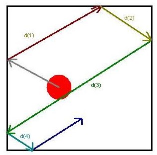
Figure \(\PageIndex{7}\): This figure shows a ball traveling in a box.

Each path traveled by the ball has a distance, denoted d_n:

\[\lambda = \dfrac{d_1 + d_2 + d_3 + d_4}{4} \label{1.2.55}\]

Calculations

In reality, the mean free path cannot be calculated by taking the average of all the paths because it is impossible to know the distance of each path traveled by a molecule. However, we can calculate it from the average speed (\(v_{\rm avg}\)) of the molecule divided by the collision frequency (\(Z\)). The formula for this is:

\[\lambda = \dfrac{v_{\rm ref}}{Z}\label{1.2.56} \]

Recall that

\[Z=\sigma v_{\rm rel}\left(\dfrac{P}{kT}\right)\tag{1.2.54} \]

therefore

\[\lambda= \left(\dfrac{kT}{\sigma P}\right)\label{1.2.57}\]

Factors affecting mean free path

• Density: As gas density increases, the molecules become closer to each other. Therefore, they are more likely to run into each other, so the mean free path decreases.
  • Increasing the number of molecules or decreasing the volume causes density to increase. This decreases the mean free path.
• Radius of molecule: Increasing the radii of the molecules decreases the space between them, causing them to run into each other more often. Therefore, the mean free path decreases.
• Pressure, temperature, and other factors that affect density can indirectly affect mean free path.

Exercise \(\PageIndex{3}\)

1. If the temperature of the system was increased, how would the collisional frequency be affected?
2. If the mass of the particles is increased, how would the collisional frequency be affected?
3. Ar gas (collision cross-section = 0.36 nm²) occupies a 1-liter (0.001m³) container at 1 atm (1.01x10⁵ kPa) of pressure and at room temperature (298K). From \(Exercise{1.2.2}\) the \(v_{\rm avg}\) for Ar at 298 K was found to be 291 m/s.

a) Calculate the mean relative speed of Ar atoms.

b) Calculate the number of collisions a single Ar atom makes in one second.(Hint: use equation \(\ref{1.2.54}\))

c) Calculate the mean free path of an argon atom.

Answers:

1. The collisional frequency decreases as temperature increases.

2. The collisional frequency decreases as the mass of the particles increases.

3.a) 412 m/s b) 3.6 x 10⁹ s^-1 c) 1.1 x 10^-7 m

Summary

• The kinetic molecular theory of gases provides a molecular explanation for the observations that led to the development of the ideal gas law.
• Average kinetic energy:\[\overline{e_K}=\dfrac{1}{2}m{v_{\rm rms}}^2=\dfrac{3}{2}\dfrac{R}{N_A}T,\label{1.2.58}\]
• Root-mean square speed: \[v_{\rm rms}=\sqrt{\dfrac{v_1^2+v_2^2+\cdots v_N^2}{N}},\label{1.2.59}\]
• Kinetic molecular theory of gases: \[v_{\rm rms}=\sqrt{\dfrac{3RT}{M}}.\label{1.2.60}\]
• Molecular motion, which leads to collisions between molecules and the container walls, explains pressure, and the large intermolecular distances in gases explain their high compressibility.
• The actual values of speed and kinetic energy are not the same for all particles of a gas but are given by a Boltzmann distribution, in which some molecules have higher or lower speeds (and kinetic energies) than average.

References

1. Dunbar, R.C. Deriving the Maxwell Distribution J. Chem. Ed. 1982, 59, 22-23.
2. Peckham, G.D.; McNaught, I.J.; Applications of the Maxwell-Boltzmann Distribution J. Chem. Ed. 1992, 69, 554-558.
3. Chang, R. Physical Chemistry for the Biosciences, 25-27.
4. https://ocw.mit.edu/courses/chemistr...lecture-notes/ (https://creativecommons.org/licenses.../4.0/legalcode)
5. Atkins, Peter and Julio de Paula. Physical Chemistry for the Life Sciences. 2006. New York, NY: W.H. Freeman and Company. pp.282-288, 290
6. Atkins, Peter. Physical Chemistry: Sixth Edition. 2000. New York, NY: W.H. Freeman and Company. pp.29,30
7. Atkins, Peter. Concepts in Physical Chemistry. 1995. New York, NY: W.H. Freeman and Company. pp.64
8. Collision frequency. Web. 14 Mar 2011. <http://www.everyscience.com/Chemistr...ses/c.1255.php>
9. James, Ames. "Problem set 1." (2011): Print.

Contributors and Attributions

• Prof. David Blauch (Davidson College)

• Stephen Lower, Professor Emeritus (Simon Fraser U.) Chem1 Virtual Textbook

• Adam Maley (Hope College), Keith Dunaway (UCD), Imteaz Siddique (UCD), Tho Nguyen, Michael Dai

• Tom Neils (Grand Rapids Community College)