8.1: Mixed States

Conceptually we are now switching gears to develop tools and ways of thinking about condensed phase problems. What we have discussed so far is the time-dependent properties of pure states, the states of a quantum system that can be characterized by a single wavefunction. For pure states one can precisely write the Hamiltonian for all particles and fields in the system of interest. These are systems that are isolated from their surroundings, or isolated systems to which we introduce a time-dependent potential. For describing problems in condensed phases, things are different. Molecules in dense media interact with one another, and as a result no two molecules have the same state. Energy placed into one degree of freedom will ultimately leak irreversibly into its environment. We cannot write down an exact Hamiltonian for these problems; however, we can concentrate on a few degrees of freedom that are observed in a measurement, and try and describe the influence of the surroundings in a statistical manner.

These observations lead to the concept of mixed states or statistical mixtures. A mixed state refers to any case in which we describe the behavior of an ensemble for which there is initially no phase relationship between the elements of the mixture. Examples include a system at thermal equilibrium and independently prepared states. For mixed states we have imperfect information about the system, and we use statistical averages in order to describe quantum observables.

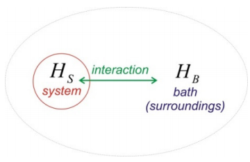
How does a system get into a mixed state? Generally, if you have two systems and you put these in contact with each other, the interaction between the two will lead to a new system that is inseparable. Consider two systems \(H_S\) and \(H_B\) for which the eigenstates of \(H_S\) are \(| n \rangle\) and those of \(H_B\) are \(| \alpha \rangle\).

\[H _ {0} = H _ {S} + H _ {B}\]

\[\left. \begin{array} {l} {H _ {S} | n \rangle = E _ {n} | n \rangle} \\ {H _ {B} | \alpha \rangle = E _ {\alpha} | \alpha \rangle} \end{array} \right. \label{0.2}\]

Before these systems interact, the state of the system \(| \psi _ {0} \rangle\) can be described as product states of \(| n \rangle\) and \(| \alpha \rangle\).

\[| \psi _ {0} \rangle = | \psi _ {S}^{0} \rangle | \psi _ {B}^{0} \rangle \label{0.3}\]

\[| \psi _ {S}^{0} \rangle = \sum _ {n} s _ {n} | n \rangle\]

\[| \psi _ {B}^{0} \rangle = \sum _ {\alpha} b _ {\alpha} | \alpha \rangle\]

\[| \psi _ {0} \rangle = \sum _ {n , \alpha} s _ {n} b _ {\alpha} | n \alpha \rangle\]

where \(s\) and \(b\) are expansion coefficients. After these states are allowed to interact, we have a new state \(| \psi (t) \rangle\). The new state can still be expressed in the zero-order basis, although this does not represent the eigenstates of the new Hamiltonian:

\[H = H _ {0} + V \label{0.6}\]

\[| \psi (t) \rangle = \sum _ {n , \alpha} c _ {n , \alpha} | n \alpha \rangle \label{0.7}\]

For any point in time, \(C _ {n , \alpha}\) is the complex amplitude for the mixed \(| n \alpha \rangle\) state. Generally speaking, at any time after bringing the systems in contact \(c _ {n , \alpha} \neq s _ {n} b _ {a}.\). The coefficient n, \(c_{n, \alpha}\) encodes \(P _ {n , \alpha} = \left| c _ {n , \alpha} \right|^{2}\), the joint probability for finding particle of \(\left|\psi_{S}\right\rangle \text {in state}|n\rangle\) and simultaneously finding particle of \(\left|\psi_{B}\right\rangle \text {in state}|\alpha\rangle\). In the case of experimental observables, we are typically able to make measurements on the system HS, and are blind to HB. Then we are interested in the probability of occupying a particular eigenstate of the system averaged over the bath degrees of freedom:

\[P _ {n} = \sum _ {\alpha} P _ {n , \alpha} = \sum _ {\alpha} \left| c _ {n , \alpha} \right|^{2} = \left\langle \left| c _ {n} \right|^{2} \right\rangle \label{0.8}\]

Now let’s look at the thinking that goes into describing ensembles. Imagine a room temperature solution of molecules dissolved in a solvent. The same molecular Hamiltonian and wavefunctions can be used to express the state of any molecule in the ensemble. However, the details of the amplitudes of the eigenstates at any moment will also depend on the timedependent local environment.

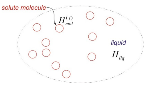
We will describe this problem with the help of a molecular Hamiltonian \(H_{m o l}^{(j)}\), which describes the state of the molecule j within the solution through the wavefunction \(\left|\psi^{(j)}\right\rangle\). We also have a Hamiltonian for the liquid \(H_{l i q}\) into which we wrap all of the solvent degrees of freedom. The full Hamiltonian for the solution can be expressed in terms of a sum over N solute molecules and the liquid, the interactions between solute molecules \(H_{i n t}\), and any solute-solvent interactions \(H_{mol-liq}\):

\[\overline {H} = \sum _ {j = 1}^{N} H _ {m o l}^{( j )} + H _ {l i q} + \sum _ {j , k = 1 \atop j > k}^{N} H _ {\text {int}}^{( j , k )} + \sum _ {j = 1}^{N} H _ {m o l - l i q}^{( j )} \label{0.9}\]

For our purposes, we take the molecular Hamiltonian to be the same for all solute molecules, i.e., \(H_{m o l}^{(j)}=H_{m o l}\) which obeys a TISE

\[H _ {m o l} | \psi _ {n} \rangle = E _ {n} | \psi _ {n} \rangle \label{0.10}\]

We will express the state of each molecule in this isolated molecule eigenbasis. For the circumstances we are concerned with, where there are no interactions or correlations between solute molecules, we are allowed to neglect \(H_{int}\). Implicit in this statement is that we believe there is no quantum mechanical phase relationship between the different solute molecules. We will also drop \(H_{liq}\), since it is not the focus of our interests and will not influence the conclusions. We can therefore write the Hamiltonian for any individual molecule as

\[H^{( j )} = H _ {m o l} + H _ {m o l - l i q}^{( j )} \label{0.11}\]

and the statistically averaged Hamiltonian

\[\overline {H} = \frac {1} {N} \sum _ {j = 1}^{N} H^{( j )} = H _ {m o l} + \left\langle H _ {m o l - l i q} \right\rangle \label{0.12}\]

This Hamiltonian reflects an ensemble average of the molecular Hamiltonian under the influence of a varying solute–solvent interaction. To describe the state of any particular molecule, we can define a molecular wavefunction \(\left|\psi_{n}^{(j)}\right\rangle\), which we express as an expansion in the isolated molecular eigenstates,

\[| \psi _ {n}^{( j )} \rangle = \sum _ {n} c _ {n}^{( j )} | \psi _ {n} \rangle \label{0.13}\]

Here the expansion coefficients vary by molecule because of their interaction with the liquid, but they are all expressed in terms of the isolated molecule eigenstates. Note that this expansion is in essence the same as Equation \ref{0.7}, with the association \(c _ {n}^{( j )} \Leftrightarrow c _ {n , \alpha}\). In either case, the mixed state arises from varying interactions with the environment. These may be static and appear from ensemble averaging, or time-dependent and arise from fluctuations in the environment. Recognizing the independence of different molecules, the wavefunction for the complete system \(|\Psi\rangle\) can be expressed in terms of the wavefunctions for the individual molecules under the influence of their local environment \(\left|\psi^{(j)}\right\rangle\):

\[\overline {H} | \Psi \rangle = \overline {E} | \Psi \rangle \label{0.14}\]

\[| \Psi \rangle = | \psi^{( 1 )} \psi^{( 2 )} \psi^{( 3 )} \cdots \rangle = \prod _ {j = 1}^{N} | \psi^{( j )} \rangle \label{0.15}\]

\[\overline {E} = \sum _ {j = 1}^{N} E^{( j )} \label{0.16}\]

We now turn out attention to expectation values that we would measure in an experiment. First we recognize that for the individual molecule j, the expectation value for an internal operator would be expressed

\[\left\langle A^{( j )} \right\rangle = \left\langle \psi^{( j )} \left| \hat {A} \left( p _ {j} , q _ {j} \right) \right| \psi^{( j )} \right\rangle \label{0.17}\]

This purely quantum mechanical quantity is itself an average. It represents the mean value obtained for a large number of measurements made on an identically prepared system, and reflects the need to average over the intrinsic quantum uncertainties in the position and momenta of particles. In the case of a mixed state, we must also average the expectation value over the ensemble of different molecules. In the case of our solution, this would involve an average of the expectation value over the N molecules.

\[\langle \langle A \rangle \rangle = \frac {1} {N} \sum _ {j = 1}^{N} \left\langle A^{( j )} \right\rangle \label{0.18}\]

Double brackets are written here to emphasize that conceptually there are two levels of statistics in this average. The first involves the uncertainty over measurements of the same molecule in the identical pure state, whereas the second is an average over variations of the state of the system within an ensemble. However, we will drop this notation when we are dealing with ensembles, and take it as understood that expectation values must be averaged over a distribution. Expanding Equation \ref{0.18} with the use of Equations \ref{0.13} and \ref{0.17} allows us to write

\[\langle A \rangle = \frac {1} {N} \sum _ {n , m} \sum _ {j = 1}^{N} c _ {m}^{( j )} \left( c _ {n}^{( j )} \right)^{*} \left\langle \psi _ {n} | \hat {A} | \psi _ {m} \right\rangle \label{0.19}\]

The second term simplifies the first expression by performing an ensemble average over the complex wavefunction amplitudes. We use this expression to write a density matrix or density operator \(\rho\), whose matrix elements are

\[\rho _ {m n} = \left\langle c _ {m} c _ {n}^{*} \right\rangle \label{0.20}\]

Then the expectation value becomes

\[\left.\begin{aligned} \langle A \rangle & = \sum _ {n , m} \rho _ {m n} A _ {n m} \\ & = \operatorname {Tr} ( \rho \hat {A} ) \end{aligned} \right. \label{0.21}\]

Here the trace \(Tr[...]\) refers to a trace over the diagonal elements of the matrix \(\sum_{a}\langle a|\cdots| a\rangle\). Although these matrices were evaluated in the basis of the molecular eigenstates, we emphasize that the definition and evaluation of the density matrix and operator matrix elements are not specific to a particular basis set.

Although this is just one example, the principles are quite generally to mixed states in the condensed phase. The wavefunction is a quantity that is meant to describe a molecular or nanoscale object. To the extent that finite temperature, fluctuations, disorder, and spatial separation ensure that phase relationships are randomized between different nano-environments, one can characterize the molecular properties of condensed phases as mixed states in which ensemble-averaging is used to describe the interactions of these molecular environments with their surroundings.

The name density matrix derives from the observation that it plays the quantum role of a probability density. Comparing Equation \ref{0.21} with the statistical determination of the mean value of \(A\),

\[\langle A \rangle = \sum _ {i = 1}^{M} P \left( A _ {i} \right) A _ {i} \label{0.22}\]

we see that \(\rho\) plays the role of the probability distribution function \(P(A)\). Since \(\rho\) is Hermitian, it can be diagonalized, and in this diagonal basis the density matrix elements are in fact the statistical weights or probabilities of occupying a given state of the system.

Returning to our example, and comparing Equation \ref{0.22} with Equation \ref{0.18} also implies that \(P_i(A) = 1/N\), i.e. that the contribution from each molecule to the average is statistically equivalent. Note also that the state of the system described by Equation \ref{0.15} is a system of fixed energy. So, the probability density in Equation \ref{0.18} indicates that this expression applies to a microcanonical ensemble (\(N\), \(V\), \(E\)) in which any realization of a system at fixed energy is equally probable, and the statistical weight is the inverse of the number of microstates: \(P=1 / \Omega\). In the case of a system in contact with a heat bath with temperature T, i.e., the canonical ensemble (N,V,T) we now express the average in terms of the probability that a member of an ensemble with fixed average energy can access a state of energy \(E\).