4.1: Introduction to Dissipative Dynamics

How does irreversible behavior, a hallmark of chemical systems, arise from the deterministic Time Dependent Schrödinger Equation? We will answer this question specifically in the context of quantum transitions from a given energy state of the system to energy states its surroundings. Qualitatively, such behavior can be expected to arise from destructive interference between oscillatory solutions of the system and the set of closely packed manifold of energy states of the bath. To illustrate this point, consider the following calculation for the probability amplitude for an initial state of the system coupled to a finite but growing number of randomly chosen states belonging to the bath.

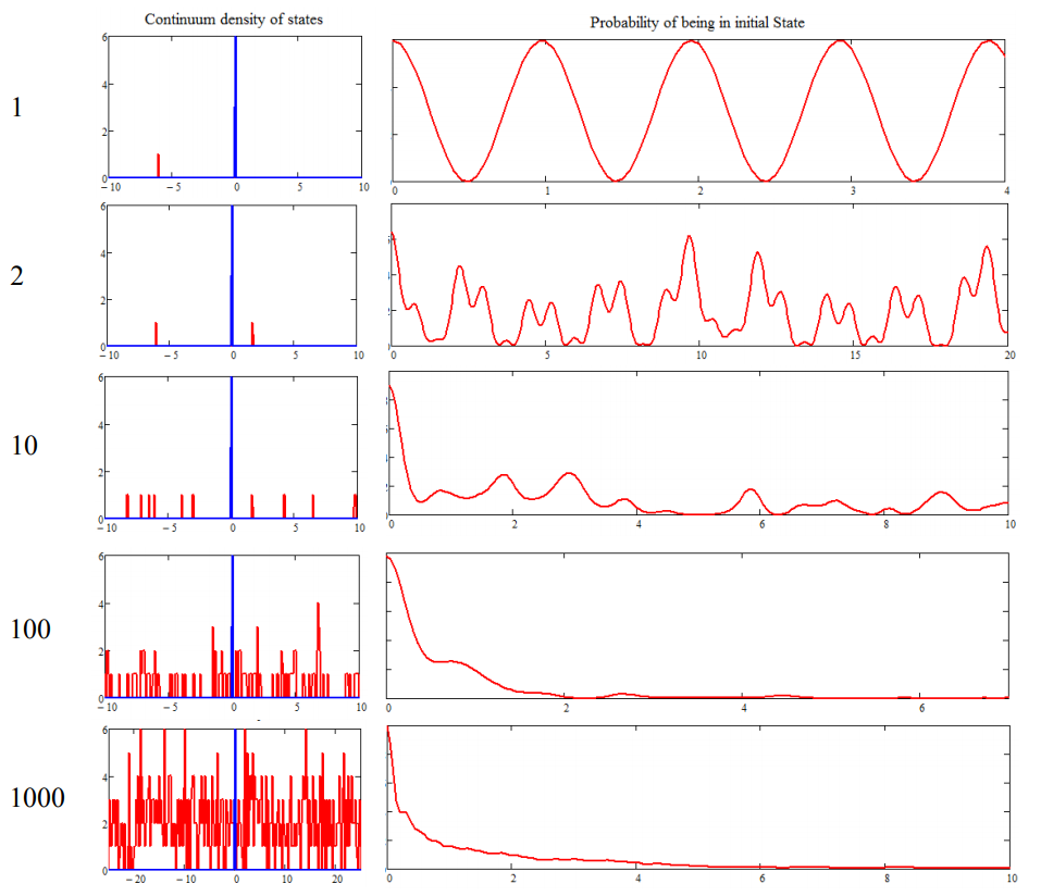
Here, even with only 100 or 1000 states, recurrences in the initial state amplitude are suppressed by destructive interference between paths. Clearly in the limit that the accepting state are truly continuous, the initial amplitude prepared in \(\ell\) will be spread through an infinite number of continuum states. We will look at this more closely by describing the relaxation of an initially prepared state as a result of coupling to a continuum of states of the surroundings. This is common to all dissipative processes in which the surroundings to the system of interest form a continuous band of states.

To begin, let us define a continuum. We are familiar with eigenfunctions being characterized by quantized energy levels, where only discrete values of the energy are allowed. However, this is not a general requirement. Discrete levels are characteristic of particles in bound potentials, but free particles can take on a continuous range of energies given by their momentum,

\[ E = \dfrac{\langle p^2 \rangle}{2m}.\]

The same applies to dissociative potential energy surfaces, and bound potentials in which the energy exceeds the binding energy. For instance, photoionization or photodissociation of a molecule involves a light field coupling a bound state into a continuum. Other examples are common in condensed matter. The intermolecular motions of a liquid, the lattice vibrations of a crystal, or the allowed energies within the band structure of a metal or semiconductor are all examples of a continuum.

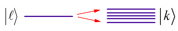
For a discrete state imbedded in such a continuum, the Golden Rule gives the probability of transition from the system state \(| \ell \rangle\) to a continuum state \(| \ell \rangle\) as:

\[\overline {w} _ {k \ell} = \frac {\partial \overline {P} _ {k \ell}} {\partial t} = \frac {2 \pi} {\hbar} \left| V _ {k \ell} \right|^{2} \rho \left( E _ {k} = E _ {\ell} \right)\]

The transition rate \(\overline {\mathcal {W}} _ {k \ell}\) is constant in time, when \(\left| V _ {k \ell} \right|^{2}\) is constant in time, which will be true for short time intervals. Under these conditions integrating the rate equation on the left gives

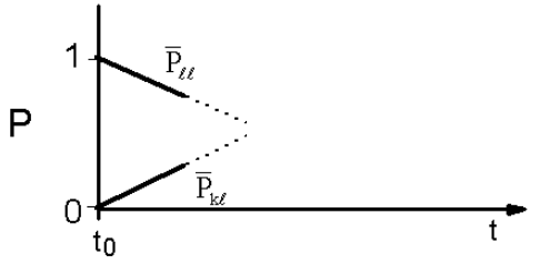
\[\begin{align} \overline {P} _ {k \ell} &= \overline {w} _ {k \ell} \left( t - t _ {0} \right) \\[4pt] \overline {P} _ {\ell \ell} &= 1 - \overline {P} _ {k \ell}. \end{align}\]

The probability of transition to the continuum of bath states varies linearly in time. As we noted, this will clearly only work for times such that

\[P _ {k} (t) - P _ {k} ( 0 ) \gg1.\]

What long time behavior do we expect? A time independent rate with population governed by

\[\overline {w} _ {k \ell} = \partial \overline {P} _ {k \ell} / \partial t\]

is a hallmark of first order kinetics and exponential relaxation. In fact, for exponential relaxation out of a state \(\ell\), the short time behavior looks just like the first order result:

\[\begin{align} \overline {P} _ {\ell \ell} (t) &= \exp \left( - \overline {w} _ {k \ell} t \right) \\ &= 1 - \overline {w} _ {k \ell} t + \ldots\label{3.4} \end{align} \]

So we might believe that \(\overline {\mathcal {W}} _ {k \ell}\) represents the tangent to the relaxation behavior at \(t - 0\). The problem we had previously was we did not account for depletion of initial state. In fact, we will see that when we look a touch more carefully, that the long time relaxation behavior of state \(\ell\) is exponential and governed by the golden rule rate. The decay of the initial state is irreversible because there is feedback with a distribution of destructively interfering phases.

Let’s formulate this problem a bit more carefully. We will look at transitions to a continuum of states \(\{k \}\) from an initial state \(\ell\) under a constant perturbation.

These together form a complete set; so for

\[H (t) = H _ {0} + V (t)\]

with \(H _ {0} | n \rangle = E _ {n} | n \rangle\).

\[1 = \sum _ {n} | n \rangle \langle n | = | \ell \rangle \left\langle \ell \left| + \sum _ {k} \right| k \right\rangle \langle k | \label{3.5}\]

As we go on, you will see that we can identify \(\ell\) with the “system” and \(\{k \}\) with the “bath” when we partition

\[H _ {0} = H _ {S} + H _ {B}.\]

Now let’s make some simplifying assumptions. For transitions into the continuum, we will assume that transitions only occur between \(\ell\) and states of the continuum, but that there are no interactions between states of the continuum: \(\left\langle k | V | k^{\prime} \right\rangle = 0\). This can be rationalized by thinking of this problem as a discrete set of states interacting with a continuum of normal modes. Moreover, we will assume that the coupling of the initial to continuum states is a constant for all states \(k\): \(\langle \ell | V | k \rangle = \left\langle \ell | V | k^{\prime} \right\rangle = \cdots\). For reasons that we will see later, we will also keep the diagonal matrix element \(\langle \ell | V | \ell \rangle = 0\). With these assumptions, we can summarize the Hamiltonian for our problem as

\begin{aligned}
H(t) &=H_{0}+V(t) \\
H_{0} &=|\ell\rangle E_{\ell}\left\langle\ell\left|+\sum_{k}\right| k\right\rangle E_{k}\langle k| \\
V(t) &=\sum_{k}\left[|k\rangle V_{k \ell}\langle\ell|+| \ell\rangle V_{2 k}\langle k|\right]+|\ell\rangle V_{\ell \ell}\langle\ell|
\label{3.6}\end{aligned}

We are seeking a more accurate description of the occupation of the initial and continuum states, for which we will use the interaction picture expansion coefficients

\[b _ {k} (t) = \left\langle k \left| U _ {I} \left( t , t _ {0} \right) \right| \ell \right\rangle \label{3.7}\]

Earlier, we saw that the exact solution to \(U_I\) was:

\[U _ {I} \left( t , t _ {0} \right) = 1 - \frac {i} {\hbar} \int _ {t _ {0}}^{t} d \tau V _ {I} ( \tau ) U _ {I} \left( \tau , t _ {0} \right) \label{3.8}\]

This form was not very practical, since \(U_I\) is a function of itself. For first-order perturbation theory, we set the final term in this equation \(U_I\), \(U _ {I} \left( \tau , t _ {0} \right) \rightarrow 1\). Here, in order to keep the feedback between \( |\ell \rangle \) and the continuum states, we keep it as is.

\[b _ {k} (t) = \langle k | \ell \rangle - \frac {i} {\hbar} \int _ {t _ {0}}^{t} d \tau \left\langle k \left| V _ {I} ( \tau ) U _ {I} \left( \tau , t _ {0} \right) \right| \ell \right\rangle \label{3.9}\]

Inserting Equation \ref{3.7}, and recognizing \(k \neq l\),

\[b _ {k} (t) = - \frac {i} {\hbar} \sum _ {n} \int _ {t _ {0}}^{t} d \tau e^{i \omega _ {h n} \tau} V _ {k n} b _ {n} ( \tau ) \label{3.10}\]

Note, \(V_{kn}\) is not a function of time. Equation \ref{3.10} expresses the occupation of state \(k\) in terms of the full history of the system from \(t _ {0} \rightarrow t\) with amplitude flowing back and forth between the states n. Equation \ref{3.10} is just the integral form of the coupled differential equations that we used before:

\[i \hbar \frac {\partial b _ {k}} {\partial t} = \sum _ {n} e^{i \omega _ {b n} t} V _ {k n} b _ {n} (t) \label{3.11}\]

These exact forms allow for feedback between all the states, in which the amplitudes \(b_k\) depend on all other states. Since you only feed from \(\ell\) into \(k\), we can remove the summation in Equation \ref{3.10} and express the complex amplitude of a state within the continuum as

\[b _ {k} = - \frac {i} {\hbar} V _ {k \ell} \int _ {t _ {0}}^{t} d \tau e^{i \omega _ {k} \tau} b _ {\ell} ( \tau ) \label{3.12}\]

We want to calculate the rate of leaving \(| \ell \rangle\), including feeding from continuum back into initial state. From Equation \ref{3.11} we can separate terms involving the continuum and the initial state:

\[i \hbar \frac {\partial} {\partial t} b _ {\ell} = \sum _ {k \neq \ell} e^{i \omega _ {\mu} t} V _ {\ell k} b _ {k} + V _ {\ell \ell} b _ {\ell} \label{3.13}\]

Now substituting Equation \ref{3.12} into Equation \ref{3.13}, and setting \(t_0 =0\):

\[\frac {\partial b _ {\ell}} {\partial t} = - \frac {1} {\hbar^{2}} \sum _ {k \neq \ell} \left| V _ {k \ell} \right|^{2} \int _ {0}^{t} b _ {\ell} ( \tau ) e^{i \omega _ {k} ( \tau - t )} d \tau - \frac {i} {\hbar} V _ {\ell \ell} b _ {\ell} (t) \label{3.14}\]

This is an integro-differential equation that describes how the time-development of \(b_ℓ\) depends on the entire history of the system. Note we have two time variables for the two propagation routes:

\[\left. \begin{array} {l} {\tau : | \ell \rangle \rightarrow | k \rangle} \\ {t : | k \rangle \rightarrow | \ell \rangle} \end{array} \right. \label{3.15}\]

The next assumption is that \(b_ℓ\) varies slowly relative to \(\omega_{kℓ}\), so we can remove it from integral. This is effectively a weak coupling statement: \(\hbar \omega _ {k \ell} \gg V _ {k \ell}\). \(b\) is a function of time, but since it is in the interaction picture it evolves slowly compared to the \(\omega_{kℓ}\) oscillations in the integral.

\[\frac {\partial b _ {\ell}} {\partial t} = b _ {\ell} \left[ - \frac {1} {\hbar^{2}} \sum _ {k \neq \ell} \left| V _ {k \ell} \right|^{2} \int _ {0}^{t} e^{i \omega _ {k} ( \tau - t )} d \tau - \frac {i} {\hbar} V _ {\ell \ell} \right] \label{3.16}\]

Now, we want the long time evolution of \(b\), for times \(\omega _ {k \ell} t > > 1\), we will investigate the integration limit \(t \rightarrow \infty\).

Note

Complex integration of Equation \ref{3.16}: Defining \(t^{\prime} = \tau - t\)

\[\int _ {0}^{t} e^{i \omega _ {k l} ( \tau - t )} d \tau = - \int _ {0}^{t} e^{i \omega _ {k l} t^{\prime}} d t^{\prime} \label{3.17}\]

The integral \(\lim _ {T \rightarrow \infty} \int _ {0}^{T} e^{i \omega t^{\prime}} d t^{\prime}\) is purely oscillatory and not well behaved. The strategy to solve this is to integrate:

\[\begin{align} \lim _ {\varepsilon \rightarrow 0^{+}} \int _ {0}^{\infty} e^{( i \omega + \varepsilon ) t^{\prime}} d t^{\prime} & = \lim _ {\varepsilon \rightarrow 0^{+}} \frac {1} {i \omega + \varepsilon} \\ & = \lim _ {\varepsilon \rightarrow 0^{+}} \left( \frac {\varepsilon} {\omega^{2} + \varepsilon^{2}} + i \frac {\omega} {\omega^{2} + \varepsilon^{2}} \right) \\ & = \pi \delta ( \omega ) - i \mathbb {P} \frac {1} {\omega} \label{3.19} \end{align}\]

(This expression is valid when used under an integral) In the final term we have written in terms of the Cauchy Principle Part:

\[\mathbb {P} \left( \frac {1} {x} \right) = \left\{\begin{array} {l l} {\frac {1} {x}} & {x \neq 0} \\ {0} & {x = 0} \end{array} \right. \label{3.20}\]

Using Equation \ref{3.19}, Equation \ref{3.16} becomes \ref{3.21}

\[\frac {\partial b _ {\ell}} {\partial t} = b _ {\ell} [ - \underbrace {\frac {\pi} {\hbar^{2}} \sum _ {k \neq \ell} \left| V _ {k \ell} \right|^{2} \delta \left( \omega _ {k \ell} \right)} _ {\text {term} 1} - \frac {i} {\hbar} \left( \underbrace {V _ {\ell \ell} + \mathbb {P} \sum _ {k \neq \ell} \frac {\left| V _ {k \ell} \right|^{2}} {E _ {k} - E _ {\ell}} )} _ {\text {term} 2} \right] \label{3.21}\]

Note that Term 1 is just the Golden Rule rate, written explicitly as a sum over continuum states instead of an integral

\[\sum _ {k \neq \ell} \delta \left( \omega _ {k \ell} \right) \Rightarrow \hbar \rho \left( E _ {k} = E _ {\ell} \right) \label{3.22}\]

\[\overline {w} _ {k \ell} = \int d E _ {k} \rho \left( E _ {k} \right) \left[ \frac {2 \pi} {\hbar} \left| V _ {k l} \right|^{2} \delta \left( E _ {k} - E _ {\ell} \right) \right] \label{3.23}\]

Term 2 is just the correction of the energy of \(E_ℓ\) from second-order time-independent perturbation theory,

\[\Delta E _ {\ell} = \langle \ell | V | \ell \rangle + \sum _ {k \neq l} \frac {\langle k | V | \left. \ell \right|^{2}} {E _ {k} - E _ {\ell}} \label{3.25} \]

So, the time evolution of \(b _ {\ell}\) is governed by a simple first-order differential equation

\[\frac{\partial b_{\ell}}{\partial t}=b_{\ell}\left(-\frac{\bar{w}_{k \ell}}{2}-\frac{i}{\hbar} \Delta E_{\ell}\right)\]

Which can be solved with \(b _ {\ell} ( 0 ) = 1\) to give

\[b _ {\ell} (t) = \exp \left( - \frac {\overline {w} _ {k l} t} {2} - \frac {i} {\hbar} \Delta E _ {\ell} t \right) \label{3.26}\]

We see that one has exponential decay of amplitude of \(b _ {\ell}\)! This is a manner of irreversible relaxation from coupling to the continuum. Now, since there may be additional interferences between paths, we switch from the interaction picture back to Schrödinger Picture,

\[c _ {\ell} (t) = \exp \left[ - \left( \frac {\overline {w} _ {k \ell}} {2} + i \frac {E _ {\ell}^{\prime}} {\hbar} \right) t \right] \label{3.27}\]

with the corrected energy

\[E _ {\ell}^{\prime} \equiv E _ {\ell} + \Delta E \label{3.28}\]

and

\[P _ {\ell} = \left| c _ {\ell} \right|^{2} = \exp \left[ - \overline {w} _ {k \ell} t \right] \label{3.29}\]

The solutions to the Time Dependent Schrödinger Equation are expected to be complex and oscillatory. What we see here is a real dissipative component and an imaginary dispersive component. The probability decays exponentially from initial state. Fermi’s Golden Rule rate tells you about long times!

Now, what is the probability of appearing in any of the states \(|k \rangle\)? Using Equation \ref{3.12}:

\[b _ {k} (t) = - \frac {i} {\hbar} \int _ {0}^{t} V _ {k \ell} e^{i \omega _ {k l} \tau} b _ {\ell} ( \tau ) d \tau\]

\[= V _ {k \ell} \frac {1 - \exp \left( - \frac {\overline {w} _ {k \ell}} {2} t - \frac {i} {h} \left( E _ {\ell}^{\prime} - E _ {k} \right) t \right)} {E _ {k} - E _ {\ell}^{\prime} + i \hbar \overline {w} _ {k \ell} / 2}\]

\[= V _ {k \ell} \frac {1 - c _ {\ell} (t)} {E _ {k} - E _ {\ell}^{\prime} + i \hbar \overline {w} _ {k \ell} / 2}\]

(3.30) If we investigate the long time limit (\(t \rightarrow \infty\)), noting that \(P _ {k \ell} = \left| b _ {k} \right|^{2}\), we find

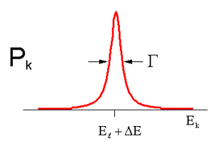
\[P _ {k l} = \frac {\left| V _ {k l} \right|^{2}} {\left( E _ {k} - E _ {i}^{\prime} \right)^{2} + \Gamma^{2} / 4} \label{3.31}\]

with

\[\Gamma \equiv \overline {w} _ {k \ell} \cdot \hbar \label{3.32}\]

The probability distribution for occupying states within the continuum is described by a Lorentzian distribution with maximum probability centered at the corrected energy of the initial state \(E _ {\ell}^{\prime}\). The width of the distribution is given by the relaxation rate, which is proxy for \(\left| V _ {k \ell} \right|^{2} \rho \left( E _ {\ell} \right)\), the coupling to the continuum and density of states.

Readings

1. Cohen-Tannoudji, C.; Diu, B.; Lalöe, F., Quantum Mechanics. Wiley-Interscience: Paris, 1977; p. 1344.
2. Merzbacher, E., Quantum Mechanics. 3rd ed.; Wiley: New York, 1998; p. 510.
3. Nitzan, A., Chemical Dynamics in Condensed Phases. Oxford University Press: New York, 2006; p. 305. 4. Schatz, G. C.; Ratner, M. A., Quantum Mechanics in Chemistry. Dover Publications: Mineola, NY, 2002; Ch. 9.