3.1: Time-Evolution Operator

Let’s start at the beginning by obtaining the equation of motion that describes the wavefunction and its time evolution through the time propagator. We are seeking equations of motion for quantum systems that are equivalent to Newton’s—or more accurately Hamilton’s—equations for classical systems. The question is, if we know the wavefunction at time \(| \psi (\vec{r}, t_o ) \rangle \), how does it change with time? How do we determine \(| \psi (\vec{r}, t ) \rangle \), for some later time \( t > t_o\)? We will use our intuition here, based largely on correspondence to classical mechanics. To keep notation to a minimum, in the following discussion we will not explicitly show the spatial dependence of wavefunction.

We start by assuming causality: \(| \psi ( t_o ) \rangle \) precedes and determines \(| \psi (t) \rangle \), which is crucial for deriving a deterministic equation of motion. Also, as usual, we assume time is a continuous variable:

\[\lim _ {t \rightarrow \tau _ {0}} | \psi (t) \rangle = | \psi \left( t _ {0} \right) \rangle \label{2.1}\]

Now define an “time-displacement operator” or “propagator” that acts on the wavefunction to the right and thereby propagates the system forward in time:

\[| \psi (t) \rangle = U \left( t , t _ {0} \right) | \psi \left( t _ {0} \right) \rangle \label{2.2}\]

We also know that the operator \(U\) cannot be dependent on the state of the system \(| \psi (t) \rangle \). This is necessary for conservation of probability, i.e., to retain normalization for the system. If

\[| \psi \left( t _ {0} \right) \rangle = a _ {1} | \varphi _ {1} \left( t _ {0} \right) \rangle + a _ {2} | \varphi _ {2} \left( t _ {0} \right) \rangle \label{2.3}\]

then

\[\begin{align} | \psi (t) \rangle & = U \left( t , t _ {0} \right) | \psi \left( t _ {0} \right) \rangle \\[4pt] & = U \left( t , t _ {0} \right) a _ {1} | \varphi _ {1} \left( t _ {0} \right) \rangle + U \left( t , t _ {0} \right) a _ {2} | \varphi _ {2} \left( t _ {0} \right) \rangle \\[4pt] & = a _ {1} (t) | \varphi _ {1} \rangle + a _ {2} (t) | \varphi _ {2} \rangle \end{align}. \label{2.4}\]

This is a reflection of the importance of linearity and the principle of superposition in quantum mechanical systems. While \(|a_i(t)|\) typically is not equal to \(|a_i(0)|\)

\[\sum _ {n} \left| a _ {n} (t) \right|^{2} = \sum _ {n} \left| a _ {n} \left( t _ {0} \right) \right|^{2} \label{2.5}\]

This dictates that the differential equation of motion is linear in time.

Properties of U

We now make some important and useful observations regarding the properties of \(U\).

1. Unitary. Note that for Equation \ref{2.5} to hold and for probability density to be conserved, \(U\) must be unitary \[P = \langle \psi (t) | \psi (t) \rangle = \left\langle \psi \left( t _ {0} \right) \left| U^{\dagger} U \right| \psi \left( t _ {0} \right) \right\rangle \label{2.6}\] which holds if \(U^{\dagger} = U^{- 1}\).
2. Time continuity: The state is unchanged when the initial and final time-points are the same \[U ( t , t ) = 1 \label{2.7}\]
3. Composition property. If we take the system to be deterministic, then it stands to reason that we should get the same wavefunction whether we evolve to a target time in one step (\(t_0 \rightarrow t_2\)) or multiple steps (\(t_0 \rightarrow t_1 \rightarrow t_2\)). Therefore, we can write \[U \left( t _ {2} , t _ {0} \right) = U \left( t _ {2} , t _ {1} \right) U \left( t _ {1} , t _ {0} \right) \label{2.8}\] Note, since \(U\) acts to the right, order matters: \[\left.\begin{aligned} | \psi \left( t _ {2} \right) \rangle & = U \left( t _ {2} , t _ {1} \right) U \left( t _ {1} , t _ {0} \right) | \psi \left( t _ {0} \right) \rangle \\[4pt] & = U \left( t _ {2} , t _ {1} \right) | \psi \left( t _ {1} \right) \rangle \end{aligned} \right. \label{2.9}\] Equation \ref{2.8} is already very suggestive of an exponential form for \(U\). Furthermore, since time is continuous and the operator is linear it it also suggests that the time propagator is only a dependent on a time interval \[U \left( t _ {1} , t _ {0} \right) = U \left( t _ {1} - t _ {0} \right) \label{2.10}\]

4. Time-reversal. The inverse of the time-propagator is the time reversal operator. From Equation \ref{2.8}:

\[ \begin{align} U \left( t , t _ {0} \right) U \left( t _ {0} , t \right) = &1 \label{2.11} \\[4pt] \therefore \,\, U^{- 1} \left( t , t _ {0} \right) &= U \left( t _ {0} , t \right) . \label{2.12} \end{align}\]

An Equation of Motion for U

Let’s find an equation of motion that describes the time-evolution operator using the change of the system for an infinitesimal time-step, \(\delta t\): \(U(t+ \delta t)\). Since

\[\lim _ {\delta t \rightarrow 0} U ( t + \delta t , t ) = 1 \label{2.13}\]

We expect that for small enough \(\delta t\), \(U\) will change linearly with \(\delta t\). This is based on analogy to thinking of deterministic motion in classical systems. Setting \(t_0\) to 0, so that \(U(t,t_o) = U(t)\), we can write

\[U ( t + \delta t ) = U (t) - i \hat {\Omega} (t) \delta t \label{2.14}\]

\(\hat{\Omega}\) is a time-dependent Hermitian operator, which is required for \(U\) to be unitary. We can now write a differential equation for the time-development of \(U(t,t_o)\), the equation of motion for \(U\):

\[\dfrac {d U (t)} {d t} = \lim _ {\delta t \rightarrow 0} \dfrac {U ( t + \delta t ) - U (t)} {\delta t} \label{2.15}\]

So from Equation \ref{2.14} we have:

\[\dfrac {\partial U \left( t , t _ {0} \right)} {\partial t} = - i \hat {\Omega} U \left( t , t _ {0} \right) \label{2.16}\]

You can now see that the operator needed a complex argument, because otherwise probability density would not be conserved; it would rise or decay. Rather it oscillates through different states of the system.

We note that \(\hat {\Omega}\) has units of frequency. Since quantum mechanics fundamentally associates frequency and energy as \(E = \hbar \omega\), and since the Hamiltonian is the operator corresponding to the energy, and responsible for time evolution in Hamiltonian mechanics, we write

\[\hat {\Omega} = \dfrac {\hat {H}} {\hbar} \label{2.17}\]

With that substitution we have an equation of motion for

\[\mathrm {i} \hbar \dfrac {\partial} {\partial t} U \left( t , t _ {0} \right) = \hat {H} U \left( t , t _ {0} \right) \label{2.18}\]

Multiplying from the right by \(| \psi(t_o) \rangle \) gives the TDSE:

\[i \hbar \dfrac {\partial} {\partial t} | \psi \rangle = \hat {H} | \psi \rangle \label{2.19}\]

If you use the Hamiltonian for a free particle (\(- \left( \hbar^{2} / 2 m \right) \left( \partial^{2} / \partial x^{2} \right)\)), this looks like a classical wave equation, except that it is linear in time. Rather, this looks like a diffusion equation with imaginary diffusion constant. We are also interested in the equation of motion for \(U^{\dagger}\) which describes the time evolution of the conjugate wavefunctions. Following the same approach and recognizing that \(U^{\dagger} \left( t , t _ {0} \right)\), acts to the left:

\[\langle \psi (t) | = \langle \psi \left( t _ {0} \right) | U^{\dagger} \left( t , t _ {0} \right) \label{2.20}\]

we get

\[- i \hbar \dfrac {\partial} {\partial t} U^{\dagger} \left( t , t _ {0} \right) = U^{\dagger} \left( t , t _ {0} \right) \hat {H} \label{2.21}\]

Evaluating the Time-Evolution Operator

At first glance it may seem straightforward to integrate Equation \ref{2.18}. If \(H\) is a function of time, then the integration of \(i \hbar \dfrac{d U}{U} = H\, dt\) gives

\[U \left( t , t _ {0} \right) = \exp \left[ \frac {- i} {\hbar} \int _ {t _ {0}}^{t} H \left( t^{\prime} \right) d t^{\prime} \right] \label{2.22}\]

Following our earlier definition of the time-propagator, this exponential would be cast as a series expansion

\[U \left( t , t _ {0} \right)^{2} = 1 - \frac {i} {\hbar} \int _ {t _ {0}}^{t} H \left( t^{\prime} \right) d t^{\prime} + \frac {1} {2 !} \left( \frac {- i} {\hbar} \right)^{2} \int _ {t _ {0}}^{t} d t^{\prime} d t^{\prime \prime} H \left( t^{\prime} \right) H \left( t^{\prime \prime} \right) + \ldots \label{2.23}\]

This approach is dangerous, since we are not properly treating \(H\) as an operator. Looking at the second term in Equation \ref{2.23}, we see that this expression integrates over both possible time-orderings of the two Hamiltonian operations, which would only be proper if the Hamiltonians at different times commute: \( H(t'),H(t'')] =0\)

Now, let’s proceed a bit more carefully assuming that the Hamiltonians at different times do not commute. Integrating Equation \ref{2.18} directly from \(t_0\) to \(t\) gives

\[U \left( t , t _ {0} \right) = 1 - \frac {i} {\hbar} \int _ {t _ {0}}^{t} d \tau H ( \tau ) U \left( \tau , t _ {0} \right) \label{2.24}\]

This is the solution; however, it is not very practical since \(U(t,t_o)\) is a function of itself. But we can make an iterative expansion by repetitive substitution of \(U\) into itself. The first step in this process is

\[\begin{align} U \left( t , t _ {0} \right) &= 1 - \frac {i} {\hbar} \int _ {t _ {0}}^{t} d \tau H ( \tau ) \left[ 1 - \frac {i} {\hbar} \int _ {t _ {0}}^{\tau} d \tau^{\prime} H \left( \tau^{\prime} \right) U \left( \tau^{\prime} , t _ {0} \right) \right] \\[4pt] & = 1 + \left( \frac {- i} {\hbar} \right) \int _ {t _ {0}}^{t} d \tau H ( \tau ) + \left( \frac {- i} {\hbar} \right)^{2} \int _ {t _ {0}}^{t} d \tau \int _ {t _ {0}}^{\tau} d \tau^{\prime} H ( \tau ) H \left( \tau^{\prime} \right) U \left( \tau^{\prime} , t _ {0} \right)\end{align} \label{2.25}\]

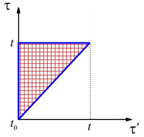
Note in the last term of this equation, that the integration limits enforce a time-ordering; that is, the first integration variable \(\tau'\) must precede the second \(\tau\). Pictorially, the area of integration is

The next substitution step gives

\[\begin{align} U \left( t , t _ {0} \right) & = 1 + \left( \frac {- i} {\hbar} \right) \int _ {t _ {0}}^{t} d \tau H ( \tau ) \nonumber \\[4pt] & + \left( \frac {- i} {\hbar} \right)^{2} \int _ {t _ {0}}^{t} d \tau \int _ {t _ {0}}^{\tau} d \tau^{\prime} H ( \tau ) H \left( \tau^{\prime} \right) \label{2.26} \\[4pt] & + \left( \frac {- i} {\hbar} \right)^{3} \int _ {t _ {0}}^{t} d \tau \int _ {t _ {0}}^{\tau} d \tau^{\prime} \int _ {t _ {0}}^{t^{\prime}} d \tau^{\prime \prime} H ( \tau ) H \left( \tau^{\prime} \right) H \left( \tau^{\prime \prime} \right) U \left( \tau^{\prime \prime} , t _ {0} \right) \nonumber \end{align}\]

From this expansion, you should be aware that there is a time-ordering to the interactions. For the third term, \(\tau^{\prime \prime}\) acts before \(\tau^{\prime}\), which acts before \(\tau\): \(t _ {0} \leq \tau^{\prime \prime} \leq \tau^{\prime} \leq \tau \leq t\)

What does this expression represent? Imagine you are starting in state \(| \psi _ {0} \rangle = | \ell \rangle\) and you want to describe how one evolves toward a target state \(| \psi \rangle = | k \rangle\). The possible paths by which one can shift amplitude and evolve the phase, pictured in terms of these time variables are:

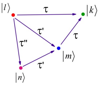
The first term in Equation \ref{2.26} represents all actions of the Hamiltonian which act to directly couple \(| \ell \rangle\) and \(| k \rangle\). The second term described possible transitions from \(| \ell \rangle\) to \(| k \rangle\) via an intermediate state \(| m \rangle\). The expression for \(U\) describes all possible paths between initial and final state. Each of these paths interferes in ways dictated by the acquired phase of our eigenstates under the timedependent Hamiltonian.

The solution for \(U\) obtained from this iterative substitution is known as the positive timeordered exponential

\[\left.\begin{aligned} U \left( t , t _ {0} \right) & = 1 + \left( \frac {- i} {\hbar} \right) \int _ {t _ {0}}^{t} d \tau H ( \tau ) \\[4pt] & + \left( \frac {- i} {\hbar} \right)^{2} \int _ {t _ {0}}^{t} d \tau \int _ {t _ {0}}^{\tau} d \tau^{\prime} H ( \tau ) H \left( \tau^{\prime} \right) \\[4pt] & + \left( \frac {- i} {\hbar} \right)^{3} \int _ {t _ {0}}^{t} d \tau \int _ {t _ {0}}^{\tau} d \tau^{\prime} \int _ {t _ {0}}^{t^{\prime}} d \tau^{\prime \prime} H ( \tau ) H \left( \tau^{\prime} \right) H \left( \tau^{\prime \prime} \right) U \left( \tau^{\prime \prime} , t _ {0} \right) \end{aligned} \right. \label{2.27}\]

(\(\hat{T}\) is known as the Dyson time-ordering operator.) In this expression the time-ordering is

\[\left. \begin{array} {l} {t _ {0} \rightarrow \tau _ {1} \rightarrow \tau _ {2} \rightarrow \tau _ {3} \dots \tau _ {n} \rightarrow t} \\[4pt] {t _ {0} \rightarrow \quad \dots \quad \tau^{\prime \prime} \rightarrow \tau^{\prime} \rightarrow \tau} \end{array} \right.\label{2.28}\]

So, this expression tells you about how a quantum system evolves over a given time interval, and it allows for any possible trajectory from an initial state to a final state through any number of intermediate states. Each term in the expansion accounts for more possible transitions between different intermediate quantum states during this trajectory.

Compare the time-ordered exponential with the traditional expansion of an exponential:

\[1 + \sum _ {n = 1}^{\infty} \frac {1} {n !} \left( \frac {- i} {\hbar} \right)^{n} \int _ {t _ {0}}^{t} d \tau _ {n} \ldots \int _ {t _ {0}}^{t} d \tau _ {1} H \left( \tau _ {n} \right) H \left( \tau _ {n - 1} \right) \ldots H \left( \tau _ {1} \right) \label{2.29}\]

Here the time-variables assume all values, and therefore all orderings for \(H(t,t_0)\) are calculated. The areas are normalized by the \(n!\) factor (there are \(n!\) time-orderings of the \(t_n\) times.) (As commented above these points need some more clarification.) We are also interested in the Hermitian conjugate of \(U \left( t , t _ {0} \right)\), which has the equation of motion in Equation \ref{2.21}. If we repeat the method above, remembering that \(U^{\dagger} \left( t , t _ {0} \right)\), acts to the left, then we obtain

\[U^{\dagger} \left( t , t _ {0} \right) = 1 + \frac {i} {\hbar} \int _ {t _ {0}}^{t} d \tau U^{\dagger} ( t , \tau ) H ( \tau ) \label{2.30}\]

Performing iterative substitution leads to a negative-time-ordered exponential:

\[U^{\dagger} \left( t , t _ {0} \right) = 1 + \frac {i} {\hbar} \int _ {t _ {0}}^{t} d \tau U^{\dagger} ( t , \tau ) H ( \tau )\label{2.31}\]

Here the \(H(\tau_i)\) act to the left.

Readings

1. Cohen-Tannoudji, C.; Diu, B.; Lalöe, F., Quantum Mechanics. Wiley-Interscience: Paris, 1977; p. 1340.
2. Merzbacher, E., Quantum Mechanics. 3rd ed.; Wiley: New York, 1998; Ch. 14.
3. Mukamel, S., Principles of Nonlinear Optical Spectroscopy. Oxford University Press: New York, 1995; Ch. 2.
4. Sakurai, J. J., Modern Quantum Mechanics, Revised Edition. Addison-Wesley: Reading, MA, 1994; Ch. 2.