16.1: Vibrational Relaxation

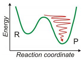
Here we want to address how excess vibrational energy undergoes irreversible energy relaxation as a result of interactions with other intra- and intermolecular degrees of freedom. Why is this process important? It is the fundamental process by which nonequilibrium states thermalize. As chemists, this plays a particularly important role in chemical reactions, where efficient vibrational relaxation of an activated species is important to stabilizing the product and not allowing it to re-cross to the reactant well. Further, the rare activation event for chemical reactions is similar to the reverse of this process. Although we will be looking specifically at vibrational couplings and relaxation, the principles are the same for electronic population relaxation through electron–phonon coupling and spin–lattice relaxation.

For an isolated molecule with few vibrational coordinates, an excited vibrational state must relax by interacting with the remaining internal vibrations or the rotational and translational degrees of freedom. If a lot of energy must be dissipated, radiative relaxation may be more likely. In the condensed phase, relaxation is usually mediated by the interactions with the environment, for instance, the solvent or lattice. The solvent or lattice forms a continuum of intermolecular motions that can absorb the energy of of the vibrational relaxation. Quantum mechanically this means that vibrational relaxation (the annihilation of a vibrational quantum) leads to excitation of solvent or lattice motion (creation of an intermolecular vibration that increases the occupation of higher lying states).

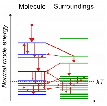
For polyatomic molecules it is common to think of energy relaxation from high lying vibrational states (\(k T \ll \hbar \omega _ {0}\)) in terms of cascaded redistribution of energy through coupled modes of the molecule and its surroundings leading finally to thermal equilibrium. We seek ways of describing these highly non-equilibrium relaxation processes in quantum systems.

Classically vibrational relaxation reflects the surroundings exerting a friction on the vibrational coordinate, which damps its amplitude and heats the sample. We have seen that a Langevin equation for an oscillator experiencing a fluctuating force \(f(t)\) describes such a process:

\[\ddot {Q} (t) + \omega _ {0}^{2} Q^{2} - \gamma \dot {Q} = f (t) / m \label{15.1}\]

This equation assigns a phenomenological damping rate \(\gamma\) to the vibrational relaxation we wish to describe. However, we know in the long time limit, the system must thermalize and the dissipation of energy is related to the fluctuations of the environment through the classical fluctuation-dissipation relationship. Specifically,

\[\langle f (t) f ( 0 ) \rangle = 2 m \gamma k _ {B} T \delta (t) \label{15.2}\]

More general classical descriptions relate the vibrational relaxation rates to the correlation function for the fluctuating forces acting on the excited coordinate.

In these classical pictures, efficient relaxation requires a matching of frequencies between the vibrational period of the excited oscillator and the spectrum of fluctuation of the environment. Since these fluctuations are dominated by motions are of the energy scale of \(k_BT\), such models do not work effectively for high frequency vibrations whose frequency \(\omega \gg k_BT/\hbar\). We would like to develop a quantum model that allows for these processes and understand the correspondence between these classical pictures and quantum relaxation.

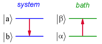
Let’s treat the problem of a vibrational system \(H_S\) that relaxes through weak coupling \(V\) to a continuum of bath states \(H_B\) using perturbation theory. The eigenstates of \(H_S\) are \(| a \rangle\) and those of \(H_B\) are \(| \alpha \rangle\). Although our earlier perturbative treatment did not satisfy energy conservation, here we can take care of it by explicitly treating the bath states.

\[\begin{align} H &= H _ {0} + V \label{15.3} \\[4pt] H _ {0} &= H _ {S} + H _ {B} \label{15.4} \end{align}\]

with

\[\begin{align} H _ {S} &= | a \rangle E _ {a} \langle a | + | b \rangle E _ {b} \langle b | \label{15.5} \\[4pt] H _ {B} &= \sum _ {\alpha} | \alpha \rangle E _ {\alpha} \langle \alpha | \label{15.6} \\[4pt] H _ {0} | a \alpha \rangle &= \left( E _ {a} + E _ {\alpha} \right) | a \alpha \rangle \label{15.7} \end{align}\]

We will describe transitions from an initial state \(| i \rangle = | a \alpha \rangle\) with energy \(E _ {a} + E _ {\alpha}\) to a final state \(| f \rangle = | b \beta \rangle\) with energy \(E _ {b} + E _ {\beta}\). Since we expect energy conservation to hold, this undoubtedly requires that a change in the system states will require an equal and opposite change of energy in the bath.

Initially, we take \(p_a=1\) and \(p_b=0\). If the interaction potential is \(V\), Fermi’s Golden Rule says the transition from \(| i \rangle\) to \(| f \rangle\) is given by

\[\begin{align} k _ {f i} &= \frac {2 \pi} {\hbar} \sum _ {i , f} p _ {i} | \langle i | V | f \rangle |^{2} \delta \left( E _ {f} - E _ {i} \right) \label{15.8} \\[4pt] &= \frac {2 \pi} {\hbar} \sum _ {a , \alpha , b , \beta} p _ {a , \alpha} | \langle a \alpha | V | b \beta \rangle |^{2} \delta \left( \left( E _ {b} + E _ {\beta} \right) - \left( E _ {a} + E _ {\alpha} \right) \right) \\[4pt] &= \frac {1} {\hbar^{2}} \int _ {- \infty}^{+ \infty} d t \sum _ {a , \alpha \atop b , \beta} p _ {a , \alpha} \langle a \alpha | V | b \beta \rangle \langle b \beta | V | a \alpha \rangle e^{- i \left( E _ {b} - E _ {a} \right) + \left( E _ {\beta} - E _ {\alpha} \right) ) t / \hbar} \label{15.10} \end{align}\]

Equation \ref{15.10} is just a restatement of the time domain version of Equation \ref{15.8}

\[k _ {f _ {f}} = \frac {1} {\hbar^{2}} \int _ {- \infty}^{+ \infty} d t \langle V (t) V ( 0 ) \rangle \label{15.11}\]

with

\[V (t) = e^{i H _ {0} t} V e^{- i H _ {0} t} \label{15.12}\]

Now, the matrix element involves both evaluation in both the system and bath states, but if we write this in terms of a matrix element in the system coordinate \(V _ {a b} = \langle a | V | b \rangle\):

\[\langle a \alpha | V | b \beta \rangle = \left\langle \alpha \left| V _ {a b} \right| \beta \right\rangle \label{15.13}\]

Then we can write the rate as

\[\begin{align} k_{b a} &=\frac{1}{\hbar^{2}} \int_{-\infty}^{+\infty} d t \sum_{\alpha, \beta} p_{\alpha}\left\langle\alpha\left|e^{+i E_{\alpha} t} V_{a b} e^{-i E_{\beta} t}\right| \beta\right\rangle\left\langle\beta\left|V_{b a}\right| \alpha\right\rangle e^{-i \omega_{b a} t} \label{15.14} \\[4pt] &=\frac{1}{\hbar^{2}} \int_{-\infty}^{+\infty} d t\left\langle V_{a b}(t) V_{b a}(0)\right\rangle_{B} e^{-i \omega_{b a} t} \label{15.15} \end{align}\]

\[V _ {a b} (t) = e^{i H _ {B} t} V _ {a b} e^{- i H _ {B} t} \label{15.16}\]

Equation \ref{15.15} says that the relaxation rate is determined by a correlation function

\[C _ {b a} (t) = \left\langle V _ {a b} (t) V _ {b a} ( 0 ) \right\rangle \label{15.17}\]

which describes the time-dependent changes to the coupling between \(b\) and \(a\). The time dependence of the interaction arises from the interaction with the bath; hence its time evolution under \(H_B\). The subscript \(\langle \cdots \rangle _ {B}\) means an equilibrium thermal average over the bath states

\[\langle \cdots \rangle _ {B} = \sum _ {\alpha} p _ {\alpha} \langle \alpha | \cdots | \alpha \rangle \label{15.18}\]

Note also that Equation \ref{15.15} is similar but not quite a Fourier transform. This expression says that the relaxation rate is given by the Fourier transform of the correlation function for the fluctuating coupling evaluated at the energy gap between the initial and final state states.

Alternatively we could think of the rate in terms of a vibrational coupling spectral density, and the rate is given by its magnitude at the system energy gap \(\omega _ {b a}\).

\[k _ {b a} = \frac {1} {\hbar^{2}} \tilde {C} _ {b a} \left( \omega _ {a b} \right) \label{15.19}\]

where the spectral representation \(\tilde {C} _ {b a} \left( \omega _ {\omega b} \right)\) is defined as the Fourier transform of \(C _ {b a} (t)\).

Vibration Coupled to a Harmonic Bath

To evaluate these expressions, let’s begin by consider the specific case of a system vibration coupled to a harmonic bath, which we will describe by a spectral density. Imagine that we prepare the system in an excited vibrational state in \(v=|1\rangle\) and we want to describe relaxation \(v=|0\rangle\).

\[H _ {S} = \hbar \omega _ {0} \left( P^{2} + Q^{2} \right) \label{15.20}\]

\[H _ {B} = \sum _ {\alpha} \hbar \omega _ {\alpha} \left( p _ {\alpha}^{2} + q _ {\alpha}^{2} \right) = \sum _ {\alpha} \hbar \omega _ {\alpha} \left( a _ {\alpha}^{\dagger} a _ {\alpha} + \frac {1} {2} \right) \label{15.21}\]

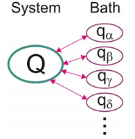
We will take the system–bath interaction to be linear in the bath coordinates:

\[V = H _ {S B} = \sum _ {\alpha} c _ {\alpha} Q q _ {\alpha} \label{15.22}\]

Here \(\mathcal {C} \alpha\) is a coupling constant which describes the strength of the interaction between the system and bath mode \(\alpha\). Note, that this form suggests that the system vibration is a local mode interacting with a set of normal vibrations of the bath.

For the case of single quantum relaxation from \(| a \rangle = | 1 \rangle\) to \(b = | 0 \rangle\), we can write the coupling matrix element as

\[V _ {b a} = \sum _ {\alpha} \xi _ {a b , \alpha} \left( a _ {\alpha}^{\dagger} + a _ {\alpha} \right) \label{15.23}\]

where

\[\xi _ {a b , \alpha} = c _ {\alpha} \frac {\sqrt {m _ {\varrho} m _ {q} \omega _ {0} \omega _ {\alpha}}} {2 \hbar} \langle b | Q | a \rangle \label{15.24}\]

Note

Note that we are using an equilibrium property, the coupling correlation function, to describe a nonequilibrium process, the relaxation of an excited state. Underlying the validity of the expressions are the principles of linear response. In practice this also implies a time scale separation between the equilibration of the bath and the relaxation of the system state. The bath correlation function should work fine if it has rapidly equilibrated, even though the system may not have. An instance where this would work well is electronic spectroscopy, where relaxation and thermalization in the excited state occurs on picosecond time scales, whereas the electronic population relaxation is on nanosecond time scales.

Here the matrix element \(\langle b | Q | a \rangle\) is taken in evaluating \(\xi _ {a b , \alpha}\). Evaluating Equation \ref{15.17} is now much the same as problems we’ve had previously:

\[\begin{align} \left\langle V _ {a b} (t) V _ {b a} ( 0 ) \right\rangle _ {B} &= \left\langle e^{i H _ {B} t} V _ {a b} e^{- i H _ {B} t} V _ {b a} \right\rangle _ {B} \\[4pt] &= \sum _ {\alpha} \xi _ {\alpha}^{2} \left[ \left( \overline {n} _ {\alpha} + 1 \right) e^{- i \omega _ {\alpha} t} + \overline {n} _ {\alpha} e^{+ i \omega _ {\alpha} t} \right] \label{15.25} \end{align}\]

here \(\overline {n} _ {\alpha} = \left( e^{\beta \hbar \omega _ {\alpha}} - 1 \right)^{- 1}\) is the thermally averaged occupation number of the bath mode at \(\omega_{\alpha}\). In evaluating this we take advantage of relationships we have used before

\[\overline {n} _ {\alpha} = \left( e^{\beta \hbar \omega _ {\alpha}} - 1 \right)^{- 1} \label{15.26}\]

\[\left. \begin{array} {l} {\left\langle a _ {\alpha} a _ {\alpha}^{\dagger} \right\rangle = \overline {n} _ {\alpha} + 1} \\ {\left\langle a _ {\alpha}^{\dagger} a _ {\alpha} \right\rangle = \overline {n} _ {\alpha}} \end{array} \right. \label{15.27}\]

So, now by Fourier transforming (Equation \ref{15.25}) we have the rate as

\[k _ {b a} = \frac {1} {\hbar^{2}} \sum _ {\alpha} \left[ \xi _ {\alpha} \right] _ {a b}^{2} \left[ \left( \overline {n} _ {\alpha} + 1 \right) \delta \left( \omega _ {b a} + \omega _ {\alpha} \right) + \overline {n} _ {\alpha} \delta \left( \omega _ {b a} - \omega _ {\alpha} \right) \right] \label{15.28}\]

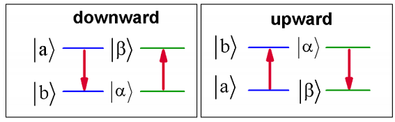
This expression describes two relaxation processes which depend on temperature. The first is allowed at \(T = 0\, K\) and is obeys \(- \omega _ {b a} = \omega _ {\alpha}\). This implies that \( E _ {a} > E _ {b} \), and that a loss of energy in the system is balanced by an equal rises in energy of the bath. That is \(| \beta \rangle = | \alpha + 1 \rangle\). The second term is only allowed for elevated temperatures. It describes relaxation of the system by transfer to a higher energy state \(E _ {b} > E _ {a}\), with a concerted decrease of the energy of the bath (\(| \beta \rangle = | \alpha - 1 \rangle\)). Naturally, this process vanishes if there is no thermal energy in the bath.

Note

There is an exact analogy between this problem and the interaction of matter with a quantum radiation field. The interaction potential is instead a quantum vector potential and the bath is the photon field of different electromagnetic modes. Equation \ref{15.28} describes has two terms that describe emission and absorption processes. The leading term describes the possibility of spontaneous emission, where a material system can relax in the absence of light by emitting a photon at the same frequency.

To more accurately model the relaxation due to a continuum of modes, we can replace the explicit sum over bath states with an integral over a density of bath states \(W\)

\[k _ {b a} = \frac {1} {\hbar^{2}} \int d \omega _ {\alpha} W \left( \omega _ {\alpha} \right) \xi _ {b a}^{2} \left( \omega _ {\alpha} \right) \left[ \left( \overline {n} \left( \omega _ {\alpha} \right) + 1 \right) \delta \left( \omega _ {b a} + \omega _ {\alpha} \right) + \overline {n} \left( \omega _ {\alpha} \right) \delta \left( \omega _ {b a} - \omega _ {\alpha} \right) \right] \label{15.29}\]

We can also define a spectral density, which is the vibrational coupling-weighted density of states:

\[\rho \left( \omega _ {\alpha} \right) \equiv W \left( \omega _ {\alpha} \right) \xi _ {b a}^{\mathcal {E}} \left( \omega _ {\alpha} \right) \label{15.30}\]

Then the relaxation rate is:

\[\left.\begin{aligned} k _ {b a} & = \frac {1} {\hbar^{2}} \int d \omega _ {\alpha} W \left( \omega _ {\alpha} \right) \xi _ {b a}^{2} \left( \omega _ {\alpha} \right) \left[ \left( \overline {n} \left( \omega _ {\alpha} \right) + 1 \right) \delta \left( \omega _ {b a} + \omega _ {\alpha} \right) + \overline {n} \left( \omega _ {\alpha} \right) \delta \left( \omega _ {b a} - \omega _ {\alpha} \right) \right] \\ & = \frac {1} {\hbar^{2}} \left[ \left( \overline {n} \left( \omega _ {b a} \right) + 1 \right) \rho _ {b a} \left( \omega _ {a b} \right) + \overline {n} \left( \omega _ {b a} \right) \rho _ {b a} \left( - \omega _ {a b} \right) \right] \end{aligned} \right. \label{15.31}\]

We see that the Fourier transform of the fluctuating coupling correlation function, is equivalent to the coupling-weighted density of states, which we evaluate at \(\omega _ {b a}\) or \(-\omega _ {b a}\) depending on whether we are looking at upward or downward transitions. Note that \(\overline {n}\) still refers to the occupation number for the bath, although it is evaluated at the energy splitting between the initial and final system states. Equation \ref{15.31} is a full quantum expression, and obeys detailed balance between the upward and downward rates of transition between two states:

\[k _ {b a} = \exp \left( - \beta \hbar \omega _ {a b} \right) k _ {a b} \label{15.32}\]

From our description of the two level system in a harmonic bath, we see that high frequency relaxation (\(k T < < \hbar \omega _ {0}\)) only proceeds with energy from the system going into a mode of the bath at the same frequency, but at lower frequencies (\(k T \approx \hbar \omega _ {0}\)) that energy can flow both into the bath and from the bath back into the system. When the vibration has energies that are thermally populated in the bath, we return to the classical picture of a vibration in a fluctuating environment that can dissipate energy from the vibration as well as giving kicks that increase the energy of the vibration. Note that in a cascaded relaxation scheme, as one approaches kT, the fraction of transitions that increase the system energy increase. Also, note that the bi-linear coupling in Equation \ref{15.22} and used in our treatment of quantum fluctuations can be associated with fluctuations of the bath that induce changes in energy (relaxation) and shifts of frequency (dephasing).

Multiquantum Relaxation of Polyatomic Molecules

3 Vibrational relaxation of polyatomic molecules in solids or in solution involves anharmonic coupling of energy between internal vibrations of the molecule, also called IVR (internal vibrational energy redistribution). Mechanical interactions between multiple modes of vibrationof the molecule act to rapidly scramble energy deposited into one vibrational coordinate and lead to cascaded energy flow toward equilibrium.

For this problem the bilinear coupling above doesn’t capture the proper relaxation process. Instead we can express the molecular potential energy in terms of well-defined normal modes of vibration for the system and the bath, and these interact weakly through small anharmonic terms in the potential. Then we can extend the perturbative approach above to include the effect of multiple accepting vibrations of the system or bath. For a set of system and bath coordinates, the potential energy for the system and system–bath interaction can be expanded as

\[V _ {S} + V _ {S B} = \frac {1} {2} \sum _ {a} \frac {\partial^{2} V} {\partial Q _ {a}^{2}} Q _ {a}^{2} + \frac {1} {6} \sum _ {a , \alpha , \beta} \frac {\partial^{3} V} {\partial Q _ {a} \partial q _ {\alpha} \partial q _ {\beta}} Q _ {a , b , \alpha} q _ {\beta} + \frac {1} {6} \sum _ {a , b , \alpha} \frac {\partial^{3} V} {\partial Q _ {a} \partial Q _ {b} \partial q _ {\alpha}} Q _ {a} Q _ {b} q _ {\alpha} \cdots \label{15.33}\]

Focusing explicitly on the first cubic expansion term, for one system oscillator:

\[V _ {S} + V _ {S B} = \frac {1} {2} m \Omega^{2} Q^{2} + V^{( 3 )} Q q _ {\alpha} q _ {\beta} \label{15.34}\]

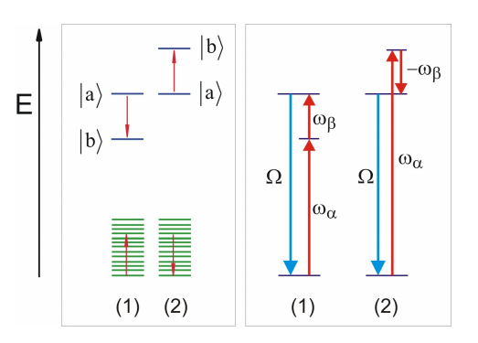
Here, the system–bath interaction potential describes the case for a cubic anharmonic coupling that involves one vibration of the system \(Q\) interacting weakly with two vibrations of the bath \(\frac {9} {2} \alpha\) and \(9 _ {\beta}\), so that \(\hbar \Omega \gg V^{( 3 )}\). Energy deposited in the system vibration will dissipate to the two vibrations of the bath, a three quantum process. Higher-order expansion terms would describe interactions involving four or more quanta.

Working specifically with the cubic example, we can use the harmonic bath model to calculate the rate of energy relaxation. This picture is applicable if a vibrational mode of frequency \(\Omega\) relaxes by transferring its energy to another vibration nearby in energy (\(\infty _ {\alpha}\)), and the energy difference \(\omega _ {\beta}\) being accounted for by a continuum of intermolecular motions. For this case one can show

\[k _ {b a} = \frac {1} {\hbar^{2}} \left[ \left( \overline {n} \left( \omega _ {\alpha} \right) + 1 \right) \left( \overline {n} \left( \omega _ {\beta} \right) + 1 \right) \rho _ {b a} \left( \omega _ {a b} \right) + \left( \overline {n} \left( \omega _ {\alpha} \right) + 1 \right) \overline {n} \left( \omega _ {\beta} \right) \rho _ {b a} \left( \omega _ {a b} \right) \right] \label{15.35}\]

where \(\rho ( \omega ) \equiv W ( \omega ) \left( V^{( 3 )} ( \omega ) \right)^{2}.\). Here we have taken , \(\Omega , \omega _ {\alpha} \gg \omega _ {\beta}\). These two terms describe two possible relaxation pathways, the first in which annihilation of a quantum of \(\Omega\) leads to a creation of one quantum each of \(\omega_{\alpha} \text { and } \omega_{\beta}\). The second term describes the dissipation of energy by coupling to a higher energy vibration, with the excess energy being absorbed from the bath. Annihilation of a quantum of \(\Omega\) leads to a creation of one quantum of \(\omega_{\alpha}\) and the annihilation of one quantum of \(\omega_{\beta}\). Naturally this latter term is only allowed when there is adequate thermal energy present in the bath.

Rate Calculations using Classical Vibrational Relaxation

In general, we would like a practical way to calculate relaxation rates, and calculating quantum correlation functions is not practical. How do we use classical calculations for the bath, for instance drawing on a classical molecular dynamics simulation? Is there a way to get a quantum mechanical rate?

The first problem is that the quantum correlation function is complex \(C _ {a b}^{*} (t) = C _ {a b} ( - t )\) and the classical correlation function is real and even \(C _ {C l} (t) = C _ {C l} ( - t )\). In order to connect these two correlation functions, one can derive a quantum correction factor that allows one to predict the quantum correlation function on the basis of the classical one. This is based on the assumption that at high temperature it should be possible to substitute the classical correlation function with the real part of the quantum correlation function

\[C _ {c} (t) \Rightarrow C _ {b n}^{\prime} (t) \label{15.36}\]

To make this adjustment we start with the frequency domain expression derived from the detailed balance expression \(\tilde {C} ( - \omega ) = e^{- \beta \hbar \omega} \tilde {C} ( \omega )\)

\[\tilde {C} ( \omega ) = \frac {2} {1 + \exp ( - \beta \hbar \omega )} \tilde {C}^{\prime} ( \omega ) \label{15.37}\]

Here \(\tilde {C}^{\prime} ( \omega )\) is defined as the Fourier transform of the real part of the quantum correlation function. So the vibrational relaxation rate is

\[k _ {b a} = \frac {4} {\hbar^{2} \left( 1 + \exp \left( - \hbar \omega _ {b a} / k T \right) \right)} \int _ {0}^{\infty} d t e^{- i \omega _ {\omega a} t} \operatorname {Re} \left[ \left\langle V _ {a b} (t) V _ {b a} ( 0 ) \right\rangle \right] \label{15.38}\]

Now we will assume that one can replace a classical calculation of the correlation function here as in Equation \ref{15.36}. The leading term out front can be considered a “quantum correction factor” that accounts for the detailed balance of rates encoded in the quantum spectral density.

In practice such a calculation might be done with molecular dynamics simulations. Here one has an explicit characterization of the intermolecular forces that would act to damp the excited vibrational mode. One can calculate the system–bath interactions by expanding the vibrational potential of the system in the bath coordinates

\[\left.\begin{aligned} V _ {S} + V _ {s B} & = V _ {0} + \sum _ {\alpha} \frac {\partial V^{\alpha}} {\partial Q} Q + \sum _ {\alpha} \frac {\partial^{2} V^{\alpha}} {\partial Q^{2}} Q^{2} + \cdots \\ & = V _ {0} + F Q + G Q^{2} + \cdots \end{aligned} \right. \label{15.39}\]

Here \(V^{\alpha}\) represents the potential of an interaction of one solvent coordinate acting on the excited vibrational system coordinate \(Q\). The second term in this expansion \(FQ\) depends linearly on the system \(Q\) and bath \(\alpha\) coordinates, and we can use variation in this parameter to calculate the correlation function for the fluctuating interaction potential. Note that \(F\) is the force that molecules exert on \(Q\)! Thus the relevant classical correlation function for vibrational relaxation is a force correlation function

\[C _ {C l} (t) = \langle F (t) F ( 0 ) \rangle \label{15.40}\]

\[k _ {C l} = \frac {1} {k T} \int _ {0}^{\infty} d t \cos \omega _ {b a} t \langle F (t) F ( 0 ) \rangle \label{15.41}\]

Readings

1. Egorov, S. A.; Rabani, E.; Berne, B. J., Nonradiative relaxation processes in condensed phases: Quantum versus classical baths. J. Chem. Phys. 1999, 110, 5238-5248.
2. Kenkre, V. M.; Tokmakoff, A.; Fayer, M. D., Theory of vibrational relaxation of polyatomic molecules in liquids. The Journal of Chemical Physics 1994, 101, 10618.
3. Nitzan, A., Chemical Dynamics in Condensed Phases. Oxford University Press: New York, 2006; Ch. 11.
4. Oxtoby, D. W., Vibrational population relaxion in liquids. Adv. Chem. Phys. 1981, 47, 487- 519.
5. Skinner, J. L., Semiclassical approximations to golden rule rate constants. The Journal of Chemical Physics 1997, 107, 8717-8718.
6. Slichter, C. P., Principles of Magnetic Resonance, with Examples from Solid State Physics. Harper & Row: New York, 1963.