14.1: Fluctuations and Randomness - Some Definitions

“Fluctuations” is my word for the time-evolution of a randomly perturbed system at or near equilibrium. For chemical problems in the condensed phase we constantly come up against the problem of random fluctuations to dynamical variables as a result of their interactions with their environment. It is unreasonable to think that you will come up with an equation of motion for the internal deterministic variable, but we should be able to understand the behavior statistically and come up with equations of motion for probability distributions. Models of this form are commonly referred to as stochastic. A stochastic equation of motion is one which includes a random component to the time-development.

When we introduced correlation functions, we discussed the idea that a statistical description of a system is commonly formulated in terms of probability distribution functions \(P\). Observables are commonly described by moments of this distribution, which are obtained by integrating over \(P\), for instance

\[\left.\begin{aligned} \langle x \rangle & = \int d x \,x \mathrm {P} (x) \\ \left\langle x^{2} \right\rangle & = \int d x \,x^{2} \mathrm {P} (x) \end{aligned} \right. \label{13.1}\]

For time-dependent processes, we recognize that it is possible that the probability distribution carries a time-dependence.

\[\begin{align} \langle x (t) \rangle & = \int d x \,x (t) \mathrm {P} ( x , t ) \\ \left\langle x^{2} (t) \right\rangle & = \int d x \,x^{2} (t) \mathrm {P} ( x , t ) \label{13.2} \end{align} \]

Correlation functions go a step further and depend on joint probability distributions \(\mathrm {P} \left( t^{\prime \prime} , A ; t^{\prime} , B \right)\) that give the probability of observing a value of \(A\) at time \(t''\) and a value of \(B\) at time \(t'\):

\[\left\langle A \left( t^{\prime \prime} \right) B \left( t^{\prime} \right) \right\rangle = \int d A \int d B \, A B \,\mathrm {P} \left( t^{\prime \prime} , A ; t^{\prime} , B \right)\label{13.3} \]

The statistical description of random fluctuations are described through these time-dependent probability distributions, and we need a stochastic equation of motion to describe their behavior. A common example of such a process is Brownian motion, the fluctuating position of a particle under the influence of a thermal environment.

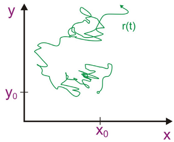
It is not practical to describe the absolute position of the particle, but we can formulate an equation of motion for the probability of finding the particle in time and space given that you know its initial position. Working from a random walk model, one can derive an equation of motion that takes the form of the well-known diffusion equation, here written in one dimension:

\[\dfrac {\partial \mathrm {P} ( x , t )} {\partial t} = \mathcal {D} \dfrac {\partial^{2}} {\partial x^{2}} \mathrm {P} ( x , t ) \label{13.4}\]

Here \(\mathcal {D}\) is the diffusion constant which sets the time scale and spatial extent of the random motion. [Note the similarity of this equation to the time-dependent Schrödinger equation for a free particle if \(\mathcal {D}\) is taken as imaginary]. Given the initial condition \(\mathrm {P} \left( x , t _ {0} \right) = \delta \left( x - x _ {0} \right)\), the solution is a conditional probability density

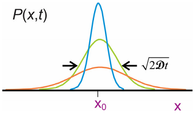
\[\mathrm {P} \left( x , t ; x _ {0} , t _ {0} \right) = \dfrac {1} {\sqrt {2 \pi \mathcal {D} \left( t - t _ {0} \right)}} \exp \left( - \dfrac {\left( x - x _ {0} \right)^{2}} {4 \mathcal {D} \left( t - t _ {0} \right)} \right) \label{13.5}\]

The probability distribution describes the statistics for fluctuations in the position of a particle averaged over many trajectories. Analyzing the moments of this probability density using Equation \ref{13.2} we find that

\[\begin{align} \langle x (t) \rangle & = x _ {0} \\[4pt] \left\langle \delta x (t)^{2} \right\rangle & = 2 \mathcal {D} t .\end{align}\]

where

\[\delta x (t) = x (t) - x _ {0}\]

So, the distribution maintains a Gaussian shape centered at \(x_0\), and broadens with time as \(2\mathcal {D}t\).

Brownian motion is an example of a Gaussian-Markovian process. Here Gaussian refers to cases in which we describe the probability distribution for a variable \(P(x)\) as a Gaussian normal distribution. Here in one dimension:

\[ \begin{align} \mathrm {P} (x) &= A e^{- \left( x - x _ {0} \right)^{2} / 2 \Delta^{2}} \\[4pt] \Delta^{2} &= \left\langle x^{2} \right\rangle - \langle x \rangle^{2} \label{13.6} \end{align}\]

The Gaussian distribution is important, because the central limit theorem states that the distribution of a continuous random variable with finite variance will follow the Gaussian distribution. Gaussian distributions also are completely defined in terms of their first and second moments, meaning that a time-dependent probability density \(P(x,t)\) is uniquely characterized by a mean value in the observable variable \(x\) and a correlation function that describes the fluctuations in \(x\). Gaussian distributions for systems at thermal equilibrium are also important for the relationship between Gaussian distributions and parabolic free energy surfaces:

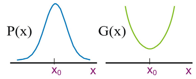
\[G (x) = - k _ {B} T \ln \mathrm {P} (x) \label{13.7}\]

If the probability density is Gaussian along \(x\), then the system’s free energy projected onto this coordinate (often referred to as a potential of mean force) has a harmonic shape. Thus Gaussian statistics are effective for describing fluctuations about an equilibrium mean value \( x_o\).

Markovian means that the time-dependent behavior of a system does not depend on its earlier history, statistically speaking. Naturally the state of any one molecule depends on its trajectory through phase space, however we are saying that from the perspective of an ensemble there is no memory of the state of the system at an earlier time. This can be stated in terms of joint probability functions as

\[\mathrm {P} \left( x _ {2} , t _ {2} ; x _ {1} , t _ {1} ; x _ {0} , t _ {0} \right) = \mathrm {P} \left( x _ {2} , t _ {2} ; x _ {1} , t _ {1} \right) \mathrm {P} \left( x _ {1} , t _ {1} ; x _ {0} , t _ {0} \right)\]

or

\[\mathrm {P} \left( t _ {2} ; t _ {1} ; t _ {0} \right) = \mathrm {P} \left( t _ {2} ; t _ {1} \right) \mathrm {P} \left( t _ {1} ; t _ {0} \right)\]

The probability of observing a trajectory that takes you from state 1 at time 1 to state 2 at time 2 does not depend on where you were at time 0. Further, given the knowledge of the probability of executing changes during a single time interval, you can exactly describe \(P\) for any time interval. Markovian therefore refers to time-dependent processes on a time scale long compared to correlation time for the internal variable that you care about. For instance, the diffusion equation only holds after the particle has experienced sufficient collisions with its surroundings that it has no memory of its earlier position and momentum: \(t > \tau_c\).

Readings

1. Nitzan, A., Chemical Dynamics in Condensed Phases. Oxford University Press: New York, 2006; Ch. 1.5 and Ch. 7.