
13.1: The Displaced Harmonic Oscillator Model
- Page ID
- 107293

Here we will discuss the displaced harmonic oscillator (DHO), a widely used model that describes the coupling of nuclear motions to electronic states. Although it has many applications, we will look at the specific example of electronic absorption experiments, and thereby gain insight into the vibronic structure in absorption spectra. Spectroscopically, it can also be used to describe wavepacket dynamics; coupling of electronic and vibrational states to intramolecular vibrations or solvent; or coupling of electronic states in solids or semiconductors to phonons. As we will see, further extensions of this model can be used to describe fundamental chemical rate processes, interactions of a molecule with a dissipative or fluctuating environment, and Marcus Theory for nonadiabatic electron transfer.
The DHO and Electronic Absorption
Molecular excited states have geometries that are different from the ground state configuration as a result of varying electron configuration. This parametric dependence of electronic energy on nuclear configuration results in a variation of the electronic energy gap between states as one stretches bond vibrations of the molecule. We are interested in describing how this effect influences the electronic absorption spectrum, and thereby gain insight into how one experimentally determines the coupling of between electronic and nuclear degrees of freedom. We consider electronic transitions between bound potential energy surfaces for a ground and excited state as we displace a nuclear coordinate \(q\). The simplified model consists of two harmonic oscillators potentials whose 0-0 energy splitting is \(E _ {e} - E _ {g}\) and which depends on \(q\). We will calculate the absorption spectrum in the interaction picture using the time-correlation function for the dipole operator.
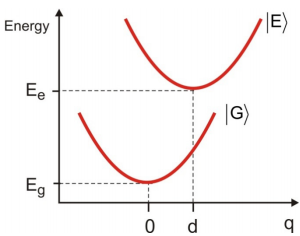
We start by writing a Hamiltonian that contains two terms for the potential energy surfaces of the electronically excited state \(| E \rangle\) and ground state \(| G \rangle\)
\[H _ {0} = H _ {G} + H _ {E} \label{12.1}\]
These terms describe the dependence of the electronic energy on the displacement of a nuclear coordinate \(q\). Since the state of the system depends parametrically on the level of vibrational excitation, we describe it using product states in the electronic and nuclear configuration, \(| \Psi \rangle = | \psi _ {\text {elec}} , \Phi _ {n u c} \rangle\), or in the present case
\[\begin{align} | G \rangle &= | g , n _ {g} \rangle \\[4pt] | E \rangle &= | e , n _ {e} \rangle \label{12.2} \end{align}\]
Implicit in this model is a Born-Oppenheimer approximation in which the product states are the eigenstates of \(H_0\), i.e.
\[H _ {G} | G \rangle = \left( E _ {g} + E _ {n _ {g}} \right) | G \rangle\]
The Hamiltonian for each surface contains an electronic energy in the absence of vibrational excitation, and a vibronic Hamiltonian that describes the change in energy with nuclear displacement.
\[\begin{align} H _ {G} & = | g \rangle E _ {g} \langle g | + H _ {g} ( q ) \\[4pt] H _ {E} & = | e \rangle E _ {e} \langle e | + H _ {e} ( q ) \label{12.3} \end{align}\]
For our purposes, the vibronic Hamiltonian is harmonic and has the same curvature in the ground and excited states, however, the excited state is displaced by d relative to the ground state along a coordinate \(q\).
\[\begin{align} H _ {g} &= \frac {p^{2}} {2 m} + \frac {1} {2} m \omega _ {0}^{2} q^{2} \label{12.4} \\[4pt] H _ {e} &= \frac {p^{2}} {2 m} + \frac {1} {2} m \omega _ {0}^{2} ( q - d )^{2} \label{12.5} \end{align}\]
The operator \(q\) acts only to changes the degree of vibrational excitation on the \(| E \rangle\) or \(| G \rangle\) surface.
We now wish to evaluate the dipole correlation function
\[\begin{align} C _ {\mu \mu} (t) & = \langle \overline {\mu} (t) \overline {\mu} ( 0 ) \rangle \\[4pt] & = \sum _ {\ell = E , G} p _ {\ell} \left\langle \ell \left| e^{i H _ {0} t / h} \overline {\mu} e^{- i H _ {0} t / h} \overline {\mu} \right| \ell \right\rangle \label{12.6} \end{align} \]
Here \(p_{\ell}\) is the joint probability of occupying a particular electronic and vibrational state, \(p _ {\ell} = p _ {\ell , e l e c} p _ {\ell , v i b}\). The time propagator is
\[e^{- i H _ {d} t / h} = | G \rangle e^{- i H _ {c} t h} \langle G | + | E \rangle e^{- i H _ {E} t / h} \langle E | \label{12.7}\]
We begin by making the Condon Approximation, which states that there is no nuclear dependence for the dipole operator. It is only an operator in the electronic states.
\[\overline {\mu} = | g \rangle \mu _ {g e} \langle e | + | e \rangle \mu _ {e g} \langle g | \label{12.8}\]
This approximation implies that transitions between electronic surfaces occur without a change in nuclear coordinate, which on a potential energy diagram is a vertical transition.
Under typical conditions, the system will only be on the ground electronic state at equilibrium, and substituting Equations \ref{12.7} and \ref{12.8} into Equation \ref{12.6}, we find:
\[C _ {\mu \mu} (t) = \left| \mu _ {e g} \right|^{2} e^{- i \left( E _ {e} - E _ {g} \right) t h} \left\langle e^{i H _ {g} t h} e^{- i H _ {\ell} t / h} \right\rangle \label{12.9}\]
Here the oscillations at the electronic energy gap are separated from the nuclear dynamics in the final factor, the dephasing function:
\[\begin{align} F (t) & = \left\langle e^{i H _ {g} t / \hbar} e^{- i H _ {c} t / h} \right\rangle \\[4pt] & = \left\langle U _ {g}^{\dagger} U _ {e} \right\rangle \label{12.10} \end{align}\]
The average \(\langle \ldots \rangle\) in Equations \ref{12.9} and \ref{12.10} is only over the vibrational states \(| n _ {g} \rangle\). Note that physically the dephasing function describes the time-dependent overlap of the nuclear wavefunction on the ground state with the time-evolution of the same wavepacket initially projected onto the excited state
\[F (t) = \left\langle \varphi _ {g} (t) | \varphi _ {e} (t) \right\rangle \label{12.11}\]
This is a perfectly general expression that does not depend on the particular form of the potential. If you have knowledge of the nuclear and electronic eigenstates or the nuclear dynamics on your ground and excited state surfaces, this expression is your route to the absorption spectrum.
For further information on this see:
- Schatz, G. C.; Ratner, M. A., Quantum Mechanics in Chemistry. Dover Publications: Mineola, NY, 2002; Ch. 9.
- Reimers, J. R.; Wilson, K. R.; Heller, E. J., Complex time dependent wave packet technique for thermal equilibrium systems: Electronic spectra. J. Chem. Phys. 1983, 79, 4749-4757. 12-4
To evaluate \(F(t)\) for this problem, it helps to realize that we can write the nuclear Hamiltonians as
\[\begin{align} H _ {g} &= \hbar \omega _ {0} \left( a^{\dagger} a + \ce{1/2} \right) \label{12.12} \\[4pt] H _ {e} &= \hat {D} H _ {g} \hat {D}^{\dagger} \label{12.13} \end{align} \]
Here \(\hat {D}\) is the spatial displacement operator
\[\hat {D} = \exp ( - i \hat {p} d / \hbar ) \label{12.14}\]
which shifts an operator in space as:
\[\hat {D} \hat {q} \hat {D}^{\dagger} = \hat {q} - d \label{12.15}\]
Note \(\hat{p}\) is only an operator in the vibrational degree of freedom. We can now express the excited state Hamiltonian in terms of a shifted ground state Hamiltonian in Equation \ref{12.13}, and also relate the time propagators on the ground and excited states
\[e^{- i H _ {c} t / h} = \hat {D} e^{- i H _ {g} t / h} \hat {D}^{\dagger} \label{12.16}\]
Substituting Equation \ref{12.16} into Equation \ref{12.10} allows us to write
\[\begin{align} F (t) & = \left\langle U _ {g}^{\dagger} e^{- i d p / h} U _ {g} e^{i d p / h} \right\rangle \\ & = \left\langle \hat {D} (t) \hat {D}^{\dagger} ( 0 ) \right\rangle \label{12.17} \end{align}\]
Equation \ref{12.17} says that the effect of the nuclear motion in the dipole correlation function can be expressed as a time-correlation function for the displacement of the vibration.
To evaluate Equation \ref{12.17} we write it as
\[F (t) = \left\langle e^{- i d \hat {p} (t) / \hbar} e^{i d \hat {p} ( 0 ) / \hbar} \right\rangle \label{12.18}\]
since
\[\hat {p} (t) = U _ {g}^{\dagger} \hat {p} ( 0 ) U _ {g} \label{12.19}\]
The time-evolution of \(\hat{p}\) is obtained by expressing it in raising and lowering operator form,
\[\hat {p} = i \sqrt {\frac {m \hbar \omega _ {0}} {2}} \left( a^{\dagger} - a \right) \label{12.20}\]
and evaluating Equation \ref{12.19} using Equation \ref{12.12}. Remembering \(a^{\dagger} a = n\), we find
\[\left. \begin{array} {l} {U _ {g}^{\dagger} a U _ {g} = e^{i n \omega _ {0} t} a e^{- i n \omega _ {0} t} = a e^{i ( n - 1 ) \omega _ {0} t} e^{- i n \omega _ {0} t} = a e^{- i \omega _ {0} t}} \\ {U _ {g}^{\dagger} a^{\dagger} U _ {g} = a^{\dagger} e^{+ i \omega _ {0} t}} \end{array} \right. \label{12.21}\]
which gives
\[\hat {p} (t) = i \sqrt {\frac {m \hbar \omega _ {0}} {2}} \left( a^{\dagger} e^{i \omega _ {0} t} - a e^{- i \omega _ {0} t} \right) \label{12.22}\]
So for the dephasing function we now have
\[F (t) = \left\langle \exp \left[ d \left( a^{\dagger} e^{i \omega _ {0} t} - a e^{- i \omega _ {0} t} \right) \right] \exp \left[ - d \left( a^{\dagger} - a \right) \right] \right\rangle \label{12.23}\]
where we have defined a dimensionless displacement variable
\[\underset{\sim}{d} = d \sqrt {\frac {m \omega _ {0}} {2 \hbar}} \label{12.24}\]
Since \(a^{\dagger}\) and \(a\) do not commute (\(\left[ a^{\dagger} , a \right] = - 1\)), we split the exponential operators using the identity
\[e^{\hat {A} + \hat {B}} = e^{\hat {A}} e^{\hat {B}} e^{- \frac {1} {2} [ \hat {A} , \hat {B} ]} \label{12.25}\]
or specifically for \(a^{\dagger}\) and \(a\),
\[e^{\lambda a^{\dagger} + \mu a} = e^{\lambda a^{\dagger}} e^{\mu a} e^{\frac {1} {2} \lambda \mu} \label{12.26}\]
This leads to
\[ F (t) = \left \langle \exp \left[ \underset{\sim}{d} \,a^{\dagger}\, e^{i \omega _ {0} t} \right] \exp \left[ - \underset{\sim}{d}\, a\, e^{- i \omega _ {0} t} \right] \exp \left[ - \frac {1} {2} \underset{\sim}{d}^{2} \right] \exp \left[ - \underset{\sim}{d}\, a^{\dagger} \right] \exp [ \underset{\sim}{d}\, a ] \exp \left[ - \frac {1} {2} \underset{\sim}{d}^{2} \right] \right \rangle \label{12.27}\]
Now to simplify our work further, let’s specifically consider the low temperature case in which we are only in the ground vibrational state at equilibrium \(| n _ {s} \rangle = | 0 \rangle\). Since \(a | 0 \rangle = 0\) and \(\langle 0 | a^{t} = 0\)
\[ \begin{align} e^{-\lambda a} | 0 \rangle &= | 0 \rangle \\[4pt] \langle 0 | e^{\lambda a^{\dagger}} &= \langle 0 | \label{12.28} \end{align} \]
and
\[F (t) = e^{- \underset{\sim}{d}^{2}} \left\langle 0 \left| \exp \left[ - \underset{\sim}{d} a e^{- i \omega _ {b} t} \right] \exp \left[ - \underset{\sim}{d} a^{\dagger} \right] \right| 0 \right \rangle \label{12.29}\]
In principle these are expressions in which we can evaluate by expanding the exponential operators. However, the evaluation becomes much easier if we can exchange the order of operators. Remembering that these operators do not commute, and using
\[e^{\hat {A}} e^{\hat {B}} = e^{\hat {B}} e^{\hat {A}} e^{- [ \hat {B} , \hat {A} ]} \label{12.30}\]
we can write
\[\begin{align} F (t) & {= e^{- \underset{\sim}{d}^{2}} \langle 0 \left| \exp \left[ - \underset{\sim}{d} a^{\dagger} \right] \exp \left[ - \underset{\sim}{d} \,a \, e^{- i \omega _ {0} t} \right] \exp \left[ \underset{\sim}{d}^{2} e^{- i \omega _ {0} t} \right] \| _ {0} \right\rangle} \\ & = \exp \left[ \underset{\sim}{d}^{2} \left( e^{- i \omega _ {0} t} - 1 \right) \right] \label{12.31} \end{align}\]
So finally, we have the dipole correlation function:
\[C _ {\mu \mu} (t) = \left| \mu _ {e g} \right|^{2} \exp \left[ - i \omega _ {e g} t + D \left( e^{- i \omega _ {v} t} - 1 \right) \right] \label{12.32}\]
\(D\) is known as the Huang-Rhys parameter (which should be distinguished from the displacement operator \(\hat{D}\)). It is a dimensionless factor related to the mean square displacement
\[D = d^{2} = \underset{\sim}{d}^{2} \frac {m \omega _ {0}} {2 \hbar} \label{12.33}\]
and therefore represents the strength of coupling of the electronic states to the nuclear degree of freedom. Note our correlation function has the form
\[C _ {\mu \mu} (t) = \sum _ {n} p _ {n} \left| \mu _ {m n} \right|^{2} e^{- i \omega _ {m n} t - g (t)} \label{12.34}\]
Here \(g(t)\) is our lineshape function
\[g (t) = - D \left( e^{- i \omega _ {0} t} - 1 \right) \label{12.35}\]
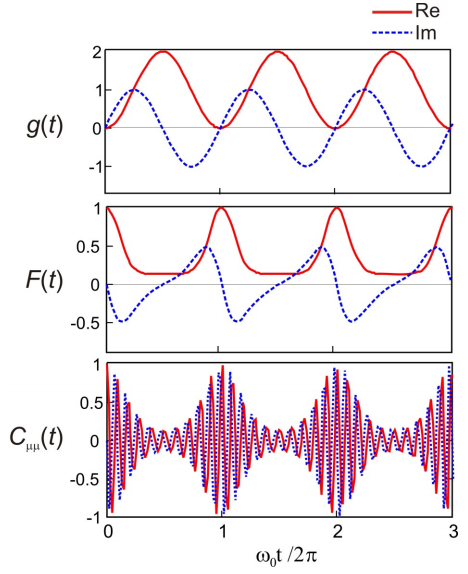
To illustrate the form of these functions, below is plotted the real and imaginary parts of \(C _ {\mu \mu} (t)\), \(F(t)\), \(g(t)\) for \(D = 1\), and \(\omega_{eg} = 10\omega_0\). \(g(t)\) oscillates with the frequency of the single vibrational mode. \(F(t)\) quantifies the overlap of vibrational wavepackets on ground and excited state, which peaks once every vibrational period. \(C _ {\mu \mu} (t)\) has the same information as \(F(t)\), but is also modulated at the electronic energy gap \(\omega_{eg}\).
Absorption Lineshape and Franck-Condon Transitions
The absorption lineshape is obtained by Fourier transforming Equation \ref{12.32}
\[\begin{align} \sigma _ {a b s} ( \omega ) & = \int _ {- \infty}^{+ \infty} d t \,e^{i \omega t} C _ {\mu \mu} (t) \\[4pt] & = \left| \mu _ {e g} \right|^{2} e^{- D} \int _ {- \infty}^{+ \infty} d t\, e^{i \omega t} e^{- i \omega _ {e s} t} \exp \left[ D e^{- i \omega _ {0} t} \right] \label{12.36} \end{align}\]
If we now expand the final term as
\[\exp \left[ D \mathrm {e}^{- i \omega _ {0} t} \right] = \sum _ {n = 0}^{\infty} \frac {1} {n !} D^{n} \left( e^{- i \omega _ {0} t} \right)^{n} \label{12.37}\]
the lineshape is
\[\sigma _ {a b s} ( \omega ) = \left| \mu _ {e g} \right|^{2} \sum _ {n = 0}^{\infty} e^{- D} \frac {D^{n}} {n !} \delta \left( \omega - \omega _ {e g} - n \omega _ {0} \right) \label{12.38}\]
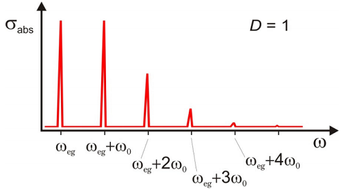
The spectrum is a progression of absorption peaks rising from \(\omega_{eg}\), separated by \(\omega_0\) with a Poisson distribution of intensities. This is a vibrational progression accompanying the electronic transition. The amplitude of each of these peaks are given by the Franck–Condon coefficients for the overlap of vibrational states in the ground and excited states
\[\left| \left\langle n _ {g} = 0 | n _ {e} = n \right\rangle \right|^{2} = | \langle 0 | \hat {D} | n \rangle |^{2} = e^{- D} \frac {D^{n}} {n !}\]
The intensities of these peaks are dependent on \(D\), which is a measure of the coupling strength between nuclear and electronic degrees of freedom. Illustrated below is an example of the normalized absorption lineshape corresponding to the correlation function for \(D = 1\) in Figure \(\PageIndex{3}\).
Now let’s investigate how the absorption lineshape depends on \(D\).
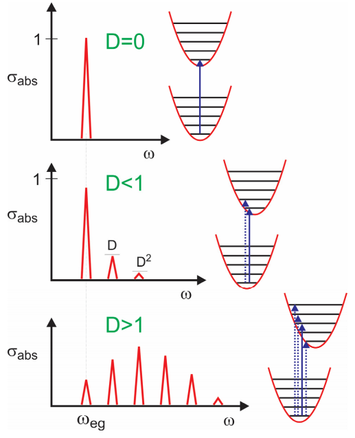
For \(D = 0\), there is no dependence of the electronic energy gap \(\omega_{eg}\) on the nuclear coordinate, and only one resonance is observed. For \(D < 1\), the dependence of the energy gap on \(q\) is weak and the absorption maximum is at \(\omega_{eg}\), with the amplitude of the vibronic progression falling off as \(D^n\). For \(D >1\), the strong coupling regime, the transition with the maximum intensity is found for peak at \(n \approx D\). So \(D\) corresponds roughly to the mean number of vibrational quanta excited from \(q = 0\) in the ground state. This is the Franck-Condon principle, that transition intensities are dictated by the vertical overlap between nuclear wavefunctions in the two electronic surfaces.
To investigate the envelope for these transitions, we can perform a short time expansion of the correlation function applicable for \(t < 1/\omega_{0}\) and for \(D \gg 1\). If we approximate the oscillatory term in the lineshape function as
\[\exp \left( - i \omega _ {0} t \right) \approx 1 - i \omega _ {0} t - \frac {1} {2} \omega _ {0}^{2} t^{2} \label{12.40}\]
then the lineshape envelope is
\[\begin{align} \sigma _ {e n v} ( \omega ) & = \left| \mu _ {e g} \right|^{2} \int _ {- \infty}^{+ \infty} d t e^{i \omega t} e^{- i \omega _ {e g} t} e^{D \left( \exp \left( - i \omega _ {0} t \right) - 1 \right)} \\ & \approx \left| \mu _ {e g} \right|^{2} \int _ {- \infty}^{+ \infty} d t e^{i \left( \omega - \omega _ {e g} t \right)} e^{D \left[ - i \omega _ {0} t - \frac {1} {2} \omega _ {0}^{2} t^{2} \right]} \\ & = \left| \mu _ {e g} \right|^{2} \int _ {- \infty}^{+ \infty} d t e^{i \left( \omega - \omega _ {e g} - D \omega _ {0} \right) t} e^{- \frac {1} {2} D \omega _ {0}^{2} t^{2}} \label{12.41} \end{align}\]
This can be solved by completing the square, giving
\[\sigma _ {e n v} ( \omega ) = \left| \mu _ {e g} \right|^{2} \sqrt {\frac {2 \pi} {D \omega _ {0}^{2}}} \exp \left[ - \frac {\left( \omega - \omega _ {e g} - D \omega _ {0} \right)^{2}} {2 D \omega _ {0}^{2}} \right] \label{12.42}\]
The envelope has a Gaussian profile which is centered at Franck–Condon vertical transition
\[\omega = \omega _ {e g} + D \omega _ {0} \label{12.43}\]
Thus we can equate \(D\) with the mean number of vibrational quanta excited in \(| E \rangle\) on absorption from the ground state. Also, we can define the vibrational energy vibrational energy in \(| E \rangle\) on excitation at \(q=0\)
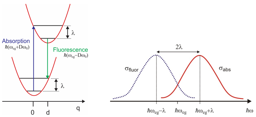
\[ \begin{align} \lambda &= D \hbar \omega _ {0} \\[4pt] &= \frac {1} {2} m \omega _ {0}^{2} d^{2} \label{12.44} \end{align}\]
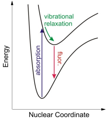
\(\lambda\) is known as the reorganization energy. This is the value of \(H_e\) at \(q=0\), which reflects the excess vibrational excitation on the excited state that occurs on a vertical transition from the ground state. It is therefore the energy that must be dissipated by vibrational relaxation on the excited state surface as the system re-equilibrates following absorption.
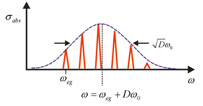
Illustration of how the strength of coupling \(D\) influences the absorption lineshape \(\sigma\) (Equation \ref{12.38}) and dipole correlation function \(C _ {\mu \mu}\) (Equation \ref{12.32}).
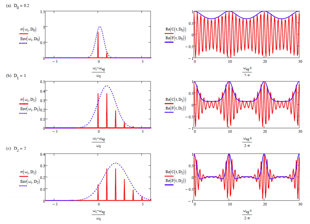
Also shown, the Gaussian approximation to the absorption profile (Equation \ref{12.42}), and the dephasing function (Equation \ref{12.31}).
Fluorescence
The DHO model also leads to predictions about the form of the emission spectrum from the electronically excited state. The vibrational excitation on the excited state potential energy surface induced by electronic absorption rapidly dissipates through vibrational relaxation, typically on picosecond time scales. Vibrational relaxation leaves the system in the ground vibrational state of the electronically excited surface, with an average displacement that is larger than that of the ground state. In the absence of other non-radiative processes relaxation processes, the most efficient way of relaxing back to the ground state is by emission of light, i.e., fluorescence. In the Condon approximation this occurs through vertical transitions from the excited state minimum to a vibrationally excited state on the ground electronic surface. The difference between the absorption and emission frequencies reflects the energy of the initial excitation which has been dissipated non-radiatively into vibrational motion both on the excited and ground electronic states, and is referred to as the Stokes shift.
From the DHO model, the emission lineshape can be obtained from the dipole correlation function assuming that the initial state is equilibrated in \(| e , 0 \rangle\), centered at a displacement \(q= d\), following the rapid dissipation of energy \(\lambda\) on the excited state. Based on the energy gap at \(q=d\), we see that a vertical emission from this point leaves \(\lambda\) as the vibrational energy that needs to be dissipated on the ground state in order to re-equilibrate, and therefore we expect the Stokes shift to be \(2\lambda\)
Beginning with our original derivation of the dipole correlation function and focusing on emission, we find that fluorescence is described by
\[\begin{align} C _ {\Omega} & = \langle e , 0 | \mu (t) \mu ( 0 ) | e , 0 \rangle = C _ {\mu \mu}^{*} (t) \\ & = \left| \mu _ {e g} \right|^{2} e^{- i \omega _ {\mathrm {g}} t} F^{*} (t) \label{12.45} \\[4pt] F^{*} (t) & = \left\langle U _ {e}^{\dagger} U _ {g} \right\rangle \\[4pt] & = \exp \left[ D \left( e^{i \omega _ {0} t} - 1 \right) \right] \label{12.46} \end{align}\]
We note that \(C _ {\mu \mu}^{*} (t) = C _ {\mu \mu} ( - t )\) and \(F^{*} (t) = F ( - t )\).
Then we can obtain the fluorescence spectrum
\[\begin{align} \sigma _ {f} ( \omega ) & = \int _ {- \infty}^{+ \infty} d t \,e^{i \omega t} C _ {\mu \mu}^{*} (t) \\[4pt] & = \left| \mu _ {e g} \right|^{2} \sum _ {n = 0}^{\infty} e^{- D} \frac {D^{n}} {n !} \delta \left( \omega - \omega _ {e g} + n \omega _ {0} \right) \end{align} \label{12.47}\]
This is a spectrum with the same features as the absorption spectrum, although with mirror symmetry about \(\omega_{eg}\).
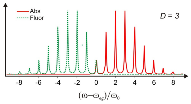
A short time expansion confirms that the splitting between the peak of the absorption and emission lineshape envelopes is \(2 D \hbar \omega_0\), or \(2\lambda\). Further, one can establish that
\[\left.\begin{aligned} \sigma _ {a b s} ( \omega ) & = \int _ {- \infty}^{+ \infty} dt\, e^{i \left( \omega - \omega _ {e g} \right) t + g (t)} \\ \sigma _ {f l} ( \omega ) & = \int _ {- \infty}^{+ \infty} dt\, e^{i \left( \omega - \omega _ {e g} \right) t + g^{*} (t)} \\ g (t) & = D \left( e^{- i \omega _ {0} t} - 1 \right) \end{aligned} \right. \label{12.48}\]
Note that our description of the fluorescence lineshape emerged from our semiclassical treatment of the light–matter interaction, and in practice fluorescence involves spontaneous emission of light into a quantum mechanical light field. However, while the light field must be handled differently, the form of the dipole correlation function and the resulting lineshape remains unchanged. Additionally, we assumed that there was a time scale separation between the vibrational relaxation in the excited state and the time scale of emission, so that the system can be considered equilibrated in \(| e , 0 \rangle\). When this assumption is not valid then one must account for the much more complex possibility of emission during the course of the relaxation process.
Readings
- Mukamel, S., Principles of Nonlinear Optical Spectroscopy. Oxford University Press: New York, 1995; p. 189, p. 217.
- Nitzan, A., Chemical Dynamics in Condensed Phases. Oxford University Press: New York, 2006; Section 12.5.
- Reimers, J. R.; Wilson, K. R.; Heller, E. J., Complex time dependent wave packet technique for thermal equilibrium systems: Electronic spectra. J. Chem. Phys. 1983, 79, 4749-4757.
- Schatz, G. C.; Ratner, M. A., Quantum Mechanics in Chemistry. Dover Publications: Mineola, NY, 2002; Ch. 9.