6.4: Adiabatic and Nonadiabatic Dynamics

The BO approximation never explicitly addresses electronic or nuclear dynamics, but neglecting the nuclear kinetic energy to obtain potential energy surfaces has implicit dynamical consequences. As we discussed for our \(\ce{NaCl}\) example, moving the neutral atoms together slowly allows electrons to completely equilibrate about each forward step, resulting in propagation on the adiabatic ground state. This is the essence of the adiabatic approximation. If you prepare the system in \(\Psi _ {\alpha}\), an eigenstate of \(H\) at the initial time \(t_0\), and propagate slowly enough, that \(\Psi _ {\alpha}\) will evolve as an eigenstate for all times:

\[H (t) \Psi _ {\alpha} (t) = E _ {\alpha} (t) \Psi _ {\alpha} (t) \label{5.15}\]

Equivalently this means that the n^th eigenfunction of \(H(t_o)\) will also be the n^th eigenfunction of \(H (t)\). In this limit, there are no transitions between BO surfaces, and the dynamics only reflect the phases acquired from the evolving system. That is the time propagator can be expressed as

\[U \left( t , t _ {0} \right) _ {a d i a b a t i c} = \sum _ {\alpha} | \alpha \rangle \langle \alpha | \exp \left( - \frac {i} {\hbar} \int _ {t _ {0}}^{t} d t^{\prime} E _ {\alpha} \left( t^{\prime} \right) \right) \label{5.16}\]

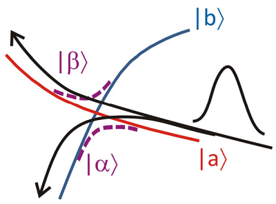
In the opposite limit, we also know that if the atoms were incident on each other so fast (with such high kinetic energy) that the electron did not have time to transfer at the crossing, that the system would pass smoothly through the crossing along the diabatic surface. In fact it is expected that the atoms would collide and recoil. This implies that there is an intermediate regime in which the velocity of the system is such that the system will split and follow both surfaces to some degree.

In a more general sense, we would like to understand the criteria for adiabaticity that enable a time-scale separation between the fast and slow degrees of freedom. Speaking qualitatively about any time-dependent interaction between quantum mechanical states, the time-scale that separates the fast and slow propagation regimes is determined by the strength of coupling between those states. We know that two coupled states exchange amplitude at a rate dictated by the Rabi frequency \(\Omega _ {R}\), which in turn depends on the energy splitting and coupling of the states. For systems in which there is significant nonperturbative transfer of population between two states \(a\) and \(b\), the time scale over which this can occur is approximately \(\Delta \mathrm {t} \approx 1 / \Omega _ {\mathrm {R}} \approx \hbar / V _ {\mathrm {ab}}\). This is not precise, but is provides a reasonable starting point for discussing “slow” versus “fast”. “Slow” in an adiabatic sense would mean that a time-dependent interaction act on the system over a period such that \(\Delta t \ll \hbar / V _ {\mathrm {ab}}\). In the case of our \(\ce{NaCl}\) example, we would be concerned with the time scale over which the atoms pass through the crossing region between diabatic states, which is determined by the incident velocity between atoms.

Adiabaticity Criterion

Let’s investigate these issues by looking more carefully at the adiabatic approximation. Since the adiabatic states (\(\Psi _ {\alpha} (t) \equiv | \alpha \rangle\)) are orthogonal for all times, we can evaluate the time propagator as

\[U (t) = \sum _ {\alpha} e^{- \frac {i} {\hbar} \int _ {0}^{t} E _ {\alpha} (t) d t^{\prime}} | \alpha \rangle \langle \alpha | \label{5.17}\]

and the time-dependent wavefunction is

\[\Psi (t) = \sum _ {\alpha} b _ {\alpha} (t) e^{- \frac {i} {\hbar} \int _ {0}^{t} E _ {\alpha} (t) d t^{\prime}} | \alpha \rangle \label{5.18}\]

Although these are adiabatic states we recognize that the expansion coefficients can be time dependent in the general case. So, we would like to investigate the factors that govern this time-dependence. To make the notation more compact, let’s define the time-rate of change of the eigenfunction as

\[| \dot {\alpha} \rangle = \frac {\partial} {\partial t} | \Psi _ {\alpha} (t) \rangle \label{5.19}\]

If we substitute the general solution Equation \ref{5.18} into the TDSE, we get

\[ i \hbar \sum _ {\alpha} \left( \dot {b} _ {\alpha} | \alpha \right\rangle + b _ {\alpha} | \dot {\alpha} \rangle - \frac {i} {\hbar} E _ {\alpha} b _ {\alpha} | \alpha \rangle ) e^{- \frac {i} {\hbar} \int _ {0}^{t} E _ {\alpha} (t) d t^{\prime}} = \sum _ {\alpha} b _ {\alpha} E _ {\alpha} | \alpha \rangle e^{- \frac {i} {\hbar} \int _ {0}^{t} E _ {\alpha} (t) d t^{\prime}} \label{5.20}\]

Note, the third term on the left hand side equals the right hand term. Acting on both sides from the left with \(\langle \beta |\) leads to

\[- \dot {b} _ {\beta} e^{- \frac {i} {h} \int _ {0}^{t} E _ {\beta} (t) d t^{\prime}} = \sum _ {\alpha} b _ {\alpha} \langle \beta | \dot {\alpha} \rangle e^{- \frac {i} {\hbar} \int _ {0}^{t} E _ {\alpha} (t) d t^{\prime}} \label{5.21}\]

We can break up the terms in the summation into one for the target state \(| \beta \rangle\) and one for the remaining states.

\[- \dot {b} _ {\beta} = b _ {\beta} \langle \beta | \dot {\beta} \rangle + \sum _ {\alpha \neq \beta} b _ {\alpha} \langle \beta | \dot {\alpha} \rangle \exp \left[ - \frac {i} {\hbar} \int _ {0}^{t} d t^{\prime} E _ {\alpha \beta} \left( t^{\prime} \right) \right] \label{5.22}\]

where

\[E _ {\alpha \beta} (t) = E _ {\alpha} (t) - E _ {\beta} (t).\]

The adiabatic approximation applies when we can neglect the summation in Equation \ref{5.22}, or equivalently when \(\langle \beta | \dot {\alpha} \rangle \ll \langle \beta | \dot {\beta} \rangle\) for all \(| \alpha \rangle\). In that case, the system propagates on the adiabatic state \(| \beta \rangle\) independent of the other states: \(\dot {b} _ {\beta} = - b _ {\beta} \langle \beta | \dot {\beta} \rangle\). The evolution of the coefficients is

\[\begin{align} b _ {\beta} (t) & = b _ {\beta} ( 0 ) \exp \left[ - \int _ {0}^{t} \left\langle \beta \left( t^{\prime} \right) | \dot {\beta} \left( t^{\prime} \right) \right\rangle d t^{\prime} \right] \\ & \approx b _ {\beta} ( 0 ) \exp \left[ \frac {i} {\hbar} \int _ {0}^{t} E _ {\beta} \left( t^{\prime} \right) d t^{\prime} \right] \label{5.23} \end{align}\]

Here we note that in the adiabatic approximation

\[E _ {\beta} (t) = \langle \beta (t) | H (t) | \beta (t) \rangle.\]

Equation \ref{5.23} indicates that in the adiabatic approximation the population in the states never changes, only their phase. The second term on the right in Equation \ref{5.22} describes the nonadiabatic effects, and the overlap integral

\[ \langle \beta | \dot {\alpha} \rangle = \left\langle \Psi _ {\beta} | \frac {\partial \Psi _ {\alpha}} {\partial t} \right\rangle \label{5.24}\]

determines the magnitude of this effect. \(\langle \beta | \dot {\alpha} \rangle\) is known as the nonadiabatic coupling (even though it refers to couplings between adiabatic surfaces), or as the geometrical phase. Note the parallels here to the expression for the nonadiabatic coupling in evaluating the validity of the BornOppenheimer approximation, however, here the gradient of the wavefunction is evaluated in time rather than the nuclear position. It would appear that we can make some connections between these two results by linking the gradient variables through the momentum or velocity of the particles involved.

So, when can we neglect the nonadiabatic effects? We can obtain an expression for the nonadiabatic coupling by expanding

\[\frac {\partial} {\partial t} [ H | \alpha \rangle = E _ {\alpha} | \alpha \rangle ] \label{5.25}\]

and acting from the left with \(\langle \beta |\), which for \(\alpha \neq \beta\) leads to

\[ \langle \beta | \dot {\alpha} \rangle = \frac {\langle \beta | \dot {H} | \alpha \rangle} {E _ {\alpha} - E _ {\beta}} \label{5.26}\]

For adiabatic dynamics to hold \(\langle \beta | \dot {\alpha} \rangle < < \langle \beta | \dot {\beta} \rangle\), and so we can say

\[\frac {\langle \beta | \dot {H} | \alpha \rangle} {E _ {\alpha} - E _ {\beta}} \ll - \frac {i} {\hbar} E _ {\beta} \label{5.27}\]

So how accurate is the adiabatic approximation for a finite time-period over which the systems propagates? We can evaluate Equation \ref{5.22}, assuming that the system is prepared in state \(| \alpha \rangle\) and that the occupation of this state never varies much from one. Then the occupation of any other state can be obtained by integrating over a period

\[\left.\begin{aligned} \dot {b} _ {\beta} & = \langle \beta | \dot {\alpha} \rangle \exp \left[ - \frac {i} {\hbar} \int _ {0}^{\tau} d t^{\prime} E _ {\alpha \beta} \left( t^{\prime} \right) \right] \\ b _ {\beta} & \approx i \hbar \frac {\langle \beta | \dot {H} | \alpha \rangle} {E _ {\alpha \beta}^{2}} \left\{\exp \left[ - \frac {i} {\hbar} E _ {\alpha \beta} \tau \right] - 1 \right\} \\ & = 2 \hbar \frac {\langle \beta | \dot {H} | \alpha \rangle} {E _ {\alpha \beta}^{2}} e^{- \frac {i} {h} E _ {\omega \beta} \tau} \sin \left( \frac {E _ {\alpha \beta} \tau} {2 \hbar} \right) \end{aligned} \right. \label{5.28}\]

Here I used

\[e^{i \theta} - 1 = 2 i e^{i \theta / 2} \sin ( \theta / 2 ).\]

For \(| b _ {\beta} k < 1\), we expand the \(\sin\) term and find

\[\left\langle \Psi _ {\beta} \left| \frac {\partial H} {\partial t} \right| \Psi _ {\alpha} \right\rangle \ll E _ {\alpha \beta} / \tau \label{5.29}\]

This is the criterion for adiabatic dynamics, which can be seen to break down near adiabatic curve crossings where \(E _ {\alpha \beta} = 0\), regardless of how fast we propagate through the crossing. Even away from curve crossing, there is always the possibility that nuclear kinetic energies are such that (\(\partial H / \partial t\)) will be greater than or equal to the energy splitting between adiabatic states.