1.4: Exponential Operators

Throughout our work, we will make use of exponential operators of the form

\[\hat {T} = e^{- i \hat {A}} \label{115}\]

We will see that these exponential operators act on a wavefunction to move it in time and space, and are therefore also referred to as propagators. Of particular interest to us is the time-evolution operator, \(\hat {U} = e^{- i \hat {H} t / \hbar},\) which propagates the wavefunction in time. Note the operator \(\hat{T}\) is a function of an operator, \(f(\hat{A})\). A function of an operator is defined through its expansion in a Taylor series, for instance

\[\hat {T} = e^{- \hat {i} \hat {A}} = \sum _ {n = 0}^{\infty} \dfrac {( - i \hat {A} )^{n}} {n !} = 1 - i \hat {\hat {A}} - \dfrac {\hat {A} \hat {A}} {2} - \cdots \label{116}\]

Since we use them so frequently, let’s review the properties of exponential operators that can be established with Equation \ref{116}. If the operator \(\hat {A}\) is Hermitian, then\(\hat {T} = e^{- i \hat {A}}\) is unitary, i.e., \(\hat {T}^{\dagger} = \hat {T}^{- 1}.\) Thus the Hermitian conjugate of \(\hat {T}\) reverses the action of \(\hat {T}\). For the time-propagator \(\vec {U}\), \(\vec {U}^{\dagger}\) is often referred to as the time-reversal operator.

The eigenstates of the operator \(\hat {A}\) also are also eigenstates of \(f(\hat {A})\), and eigenvalues are functions of the eigenvalues of \(\hat {A}\). Namely, if you know the eigenvalues and eigenvectors of \(\hat {A}\), i.e., \(\hat {A} \varphi _ {n} = a _ {n} \varphi _ {n},\)you can show by expanding the function

\[f ( \hat {A} ) \varphi _ {n} = f \left( a _ {n} \right) \varphi _ {n} \label{117}\]

Our most common application of this property will be to exponential operators involving the Hamiltonian. Given the eigenstates \(\varphi _ {n}\), then \(\hat {H} | \varphi _ {n} \rangle = E _ {n} | \varphi _ {n} \rangle\) implies

\[e^{- i \hat {H} t / \hbar} | \varphi _ {n} \rangle = e^{- i E _ {n} t / \hbar} | \varphi _ {n} \rangle \label{118}\]

Just as \(\hat {D} _ {x} ( \lambda )\) is the time-evolution operator that displaces the wavefunction in time, \(\hat {D} _ {x} = e^{- i \hat {p} _ {x} x / h}\) is the spatial displacement operator that moves \(\psi\) along the \(x\) coordinate. If we define \(\hat {D}_ {x} = e^{- i \hat {p} _ {x} x / h},\) then the action of is to displace the wavefunction by an amount \(\lambda\)

\[| \psi ( x - \lambda ) \rangle = \hat {D} _ {x} ( \lambda ) | \psi (x) \rangle \label{119}\]

Also, applying \(\hat {D} _ {x} ( \lambda )\) to a position operator shifts the operator by \(\lambda\)

\[\hat {D} _ {x}^{\dagger} \hat {x} \hat {D} _ {x} = x + \lambda \label{120}\]

Thus \(e^{- i \hat {p} _ {x} \lambda / \hbar} | x \rangle\) is an eigenvector of \(\hat {x}\) with eigenvalue \(x + \lambda\) instead of \(x\). The operator

\(\hat {D} _ {x} = e^{- i \hat {p} _ {x} \lambda / h}\) is a displacement operator for \(x\) position coordinates. Similarly, \(\hat {D} _ {y} = e^{- i \hat {p} _ {y} \lambda / h}\)generates displacements in \(y\) and \(\hat {D_z}\) in \(z\). Similar to the time-propagator \(\boldsymbol {U}\), the displacement operator \(\boldsymbol {D}\) must be unitary, since the action of \(\hat {D}^{\dagger} \hat {D}\) must leave the system unchanged. That is if \(\hat {D} _ {x}\) shifts the system to \(x\) from \(x_0\), then \(\hat {D} _ {x}^{\dagger}\) shifts the system from \(x\) back to \(x_0\).

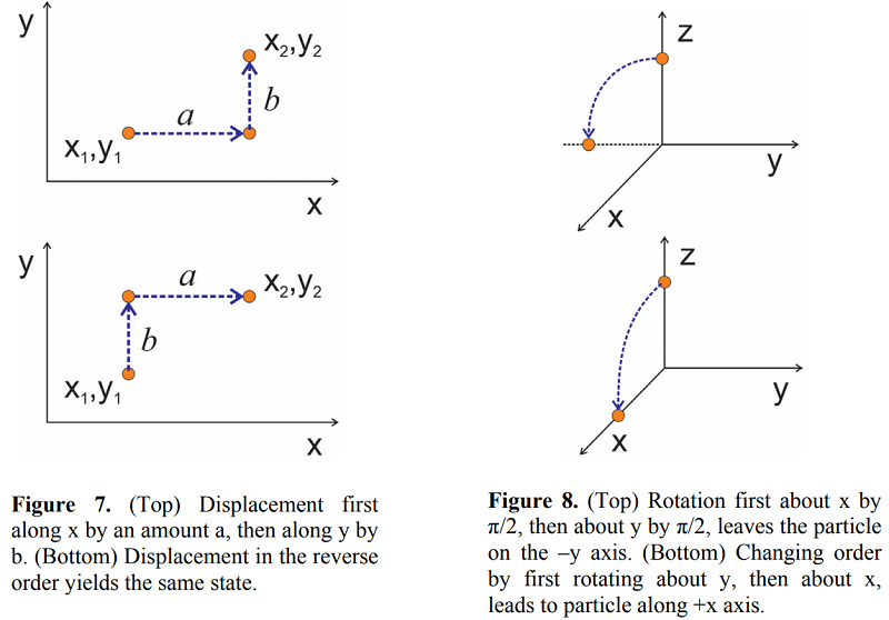
We know intuitively that linear displacements commute. For example, if we wish to shift a particle in two dimensions, x and y, the order of displacement does not matter. We end up at the same position, whether we move along x first or along y, as illustrated in Figure 7. In terms of displacement operators, we can write

\[\begin{aligned}
\left|x_{2}, y_{2}\right\rangle &=e^{-i b p_{y} / \hbar} e^{-i a p_{x} / \hbar}\left|x_{1}, y_{1}\right\rangle \\
&=e^{-i a p_{x} / \hbar} e^{-i b p_{y} / \hbar}\left|x_{1}, y_{1}\right\rangle
\end{aligned}\]

These displacement operators commute, as expected from \([p_x,p_y] = 0.\)

Similar to the displacement operator, we can define rotation operators that depend on the angular momentum operators, \(L_x\), \(L_y\), and \(L_z\). For instance,

\[\hat {R} _ {x} ( \phi ) = e^{- i \phi L _ {x} / \hbar}\]

gives a rotation by angle \(\phi\) about the \(x\) axis. Unlike linear displacement, rotations about different axes do not commute. For example, consider a state representing a particle displaced along the z axis, \(| z 0 \rangle\). Now the action of two rotations \(\hat {R} _ {x}\) and \(\hat {R} _ {y}\) by an angle of \(\phi = \pi / 2\) on this particle differs depending on the order of operation, as illustrated in Figure 8. If we rotate first about \(x\), the operation

\[e^{- i \tfrac {\pi} {2} L _ {y} / \hbar} e^{- i \tfrac {\pi} {2} L _ {x} / \hbar} | z _ {0} \rangle \rightarrow | - y \rangle \label{122}\]

leads to the particle on the –y axis, whereas the reverse order

\[e^{- i \tfrac {\pi} {2} L _ {x} / \hbar} e^{- i \tfrac {\pi} {2} L _ {y} / \hbar} | z _ {0} \rangle \rightarrow | + x \rangle \label{123}\]

leads to the particle on the +x axis. The final state of these two rotations taken in opposite order differ by a rotation about the z axis. Since rotations about different axes do not commute, we expect the angular momentum operators not to commute. Indeed, we know that

\[\left[ L _ {x} , L _ {y} \right] = i \hbar L _ {z}\]

where the commutator of rotations about the x and y axes is related by a z-axis rotation. As with rotation operators, we will need to be careful with time-propagators to determine whether the order of time-propagation matters. This, in turn, will depend on whether the Hamiltonians at two points in time commute.