7.4: Exact Differentials and State Functions

Now, let us consider the general case of a continuous function \(f\left(x,y\right)\), for which the exact differential is

\[df=f_x\left(x,y\right)dx+f_y\left(x,y\right)dy. \nonumber \]

We want to integrate the exact differential over very short paths like paths a and b in Section 7.3. Let us evaluate the integral between \(\left(x_0,y_0\right)\) and \(\left(x_0+\Delta x,y_0+\Delta y\right)\) over the paths a* and b* sketched in Figure 3.

Figure 3. Alternative paths from (\(x_0, ~ y_0\)) to (\(x_0 + \Delta x, ~ y_0 + \Delta y\))

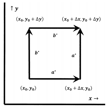
• Path a* has two linear segments. The first segment is the portion of the line \({y=y}_0\) as \(x\) goes from \(x_0\) to \(x_0+\Delta x\). Along the first segment \(\Delta y=0\). The second segment is the portion of the line \({x=x}_0+\Delta x\) as \(y\) goes from \(y_0\) to \(y_0+\Delta y\). Along the second segment, \(\Delta x=0\).
• Path b* has two linear segments also. The first segment is the portion of the line \(x=x_0\) as \(y\) goes from \(y_0\) to \(y_0+\Delta y\). Along the first segment, \(\Delta x=0\). The second segment is the portion of the line \({y=y}_0+\Delta y\) as \(x\) goes from \(x_0\) to \(x_0+\Delta x\). Along the second segment, \(\Delta y=0\).

Along path a*, we have

\[{\Delta }_{a^*}f=f_x\left(x_0,y_0\right)\Delta x+f_y\left(x_0+\Delta x,y_0\right)\Delta y\nonumber \]

Along path b*,

\[{\Delta }_{b^*}f=f_x\left(x_0,y_0+\Delta y\right)\Delta x+f_y\left(x_0,y_0\right)\Delta y\nonumber \]

In the limit as \(\Delta x\) and \(\Delta y\) become arbitrarily small, we must have \({\Delta }_{a^*}f={\Delta }_{b^*}f\), so that

\[f_x\left(x_0,y_0\right)\Delta x+f_y\left(x_0+\Delta x,y_0\right)\Delta y=f_x\left(x_0,y_0+\Delta y\right)\Delta x+f_y\left(x_0,y_0\right)\Delta y\nonumber \]

Rearranging this equation so that terms in \(f_x\) are on one side and terms in \(f_y\) are on the other side, dividing both sides by \(\Delta x\Delta y\), and taking the limit as \(\Delta x\to 0\) and \(\Delta y\to 0\), we have

\[{\mathop{\mathrm{lim}}_{\Delta x\to 0} \left[\frac{f_y\left(x_0+\Delta x,y_0\right)-f_y\left(x_0,y_0\right)}{\Delta x}\right]\ }={\mathop{\mathrm{lim}}_{\Delta y\to 0} \left[\frac{f_x\left(x_0,y_0+\Delta y\right)-f_x\left(x_0,y_0\right)}{\Delta y}\right]\ }\nonumber \]

These limits are the partial derivative of \(f_y\left(x_0,y_0\right)\) with respect to \(x\) and of \(f_x\left(x_0,y_0\right)\) with respect to \(y\). That is

\[{\left[{\frac{\partial }{\partial x}f}_y\left(x_0,y_0\right)\right]}_y={\left[\frac{\partial }{\partial x}\left(\frac{\partial f\left(x_0,y_0\right)}{\partial y}\right)\right]}_y=\frac{{\partial }^2f\left(x_0,y_0\right)}{\partial y\partial x}\nonumber \] and \[{\left[{\frac{\partial }{\partial y}f}_x\left(x_0,y_0\right)\right]}_x={\left[\frac{\partial }{\partial y}\left(\frac{\partial f\left(x_0,y_0\right)}{\partial x}\right)\right]}_x=\frac{{\partial }^2f\left(x_0,y_0\right)}{\partial x\partial y}\nonumber \]

This shows that, if \(f\left(x,y\right)\) is a continuous function of \(x\) and \(y\) whose partial derivatives exist, then

\[\frac{{\partial }^2f\left(x_0,y_0\right)}{\partial y\partial x}=\frac{{\partial }^2f\left(x_0,y_0\right)}{\partial x\partial y}\nonumber \]

The mixed second partial derivative of \(f\left(x,y\right)\) is independent of the order of differentiation. We also write these second partial derivatives as \(f_{xy}\left(x_0,y_0\right)\) and \(f_{yx}\left(x_0,y_0\right)\).

To summarize these points, if \(f\left(x,y\right)\) is a continuous function of \(x\) and \(y\), all of the following are true:

1. \(f\left(x,y\right)\) represents a surface in a three-dimensional space.
2. \(f\left(x,y\right)\) is a state function.
3. The total differential is \[df={\left({\partial f}/{\partial x}\right)}_ydx+{\left({\partial f}/{\partial y}\right)}_xdy.\nonumber \]
4. The total differential is exact.
5. The line integral of \(df\) between two points is independent of the path of integration.
6. The line integral of \(df\) around any closed path is zero: \(\oint{df=0}\).
7. The mixed second-partial derivatives are equal; that is, \[\frac{{\partial }^2f}{\partial y\partial x}=\frac{{\partial }^2f}{\partial x\partial y}\nonumber \]